Integrating an Online Portfolio Selection Model into a Trading Algorithm


Please note that this article is for educational purposes only. Alpaca does not recommend any specific securities or investment strategies.
Table of Contents
1). Background2). Online Portfolio Selection3). Selecting Best Performer Stock4). Walk Forward Optimization5). Statistical Properties of the Algorithms6). ConclusionBackground
Quantonomy LLC was founded in 2018 based on several years of experience in creating trading and mathematical models of cryptocurrencies and other financial assets. Here at Quantonomy we create algorithms for trading stocks through our AlphaHub platform which is open to early adopters. In addition to that, Quantonomy offers a Fully Automated Trader, known as AlphaHub Trader, downloadable here:
https://github.com/gsantostasi/AlphaHubTrader
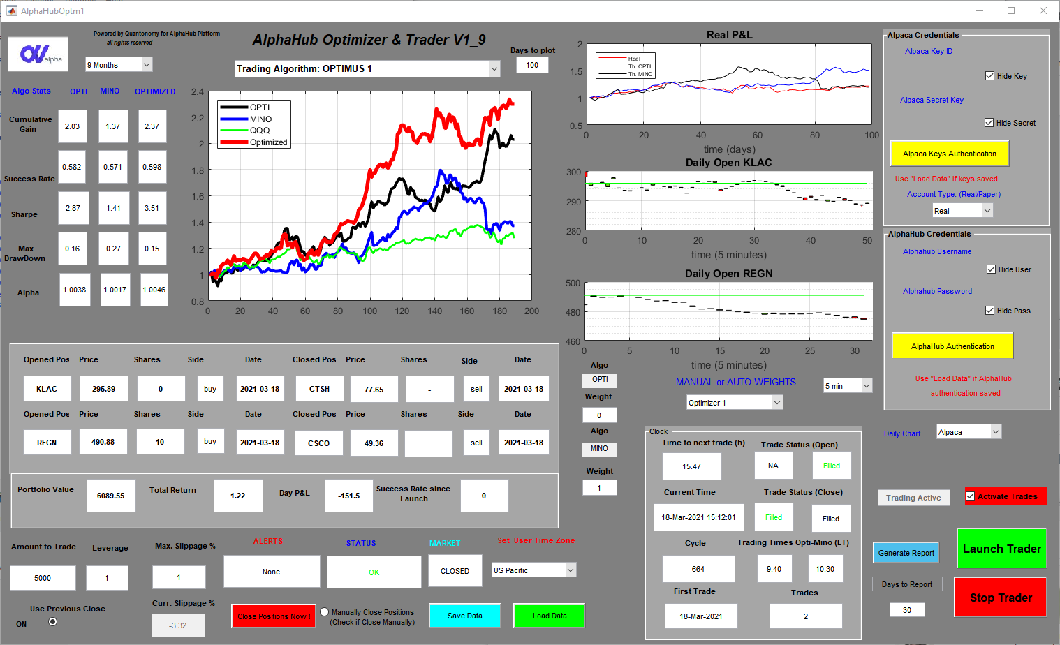
The Automated AlphaHub Trader is a .exe app that can be run on any Windows OS machine. It has an easy-to-use GUI that connects, via encrypted keys, with our chosen broker Alpaca Markets that has a user-friendly, modern, and well-documented API. Users open an individual account on Alpaca (Quantonomy has no access to the fund or the API keys) and then connect the Trader to the account.

The Trader executes the signals posted on the AlphaHub platform without any human intervention and keeps track of its performance (i.e. real trades vs theoretical performance) and produces reports that measure slippage, the average time to execute a trade, and other algo behavioral parameters.
Now Let's Start
I’m the Chief Scientific Officer of Quantonomy. I have worked in several fields of science. I gained my Ph.D. in Physics with a dissertation on Gravitational Waves and the physics of neutron stars. In 2009, for several professional and personal reasons, I switched to the field of neuroscience and made important contributions in the Neuroscience of Sleep and I even patented a method to enhance memory and cognition during the most restorative part of sleep, called Slow Wave Sleep [1].
Since 2012 I have been interested in cryptocurrencies and I noticed particular mathematical patterns in the price of Bitcoin. I have been one of the first people posting publicly on this topic in particular on Facebook (on several BTC-related groups) and on Reddit with the user's name Econophysicist1. For example, this was one of the earliest posts on this topic [2]:

I will elaborate more on BTC mathematical behavior in subsequent articles.
Eventually, I started to study other cryptocurrencies and decided to use some of the time series tools I applied over the years to analyze scientific data in several fields to model these assets behavior.
Financial markets and physical systems bear many similarities, and many of the mathematical techniques used in predictive modeling of physical systems have proven highly applicable to financial markets [3].
In the meanwhile, other people joined my research work on cryptocurrencies and we founded Quantonomy LLC to organize more professionally this activity.
Applying principles from econophysics we started to obtain very promising results almost immediately.
During the cryptocurrency bubble of 2017, one of our algorithms gained an astonishing 6x return in a single month trading a portfolio of 16 coins.
The crash of the entire crypto market during early 2018 pushed us to adapt our algorithms to deal with a downtrend market. Our algorithms were still doing well but our particular approach of using a relatively large portfolio of coins needed a level of liquidity that the crypto market didn’t have anymore, in particular in the case of the medium or small-cap coins in our portfolio.
We decide to test very aggressive algorithms we developed explicitly for cryptocurrency trading to the stock market. We expected less volatility and our algorithms were optimized to leverage volatility to obtain consistent cumulative gains. Therefore, we were not certain our algorithms could work well in this new environment.
The algorithms, with some minor modifications, were still doing very well when relatively volatile stocks were used. NASDAQ stocks, for example, seem to work better than the ones in the S&P 500 index.
Online Portfolio Selection
After extensive research in algorithmic trading, we decided to explore one of the approaches that seemed more promising. A very active field of research in algorithmic trading centers around the use of machine learning and AI. We decided to avoid too complex methods like Deep Learning that is very interesting in theoretical terms but it is prone to many possible downfalls, in particular the problem of overfitting. We will publish other articles in the future to discuss in-depth this issue.
But in general, overfitting is a common problem in forecast modeling. When we create such models we use past trends to make inferences on the future. This is a common problem in physics, we collect data on the orbit of a newly discovered comet for example and we predict (with incredible precision) the path of the object around the sun. In physics, this works well because while the orbit can be influenced by the gravity of all the objects in the solar system most of the behavior of the comet can be explained by the gravity field of the sun and few large planets. Then we can apply well-known equations of Newtonian classical physics and extrapolate the orbit in the future.
When we deal with more random systems we can still apply a similar approach but there are no known theoretical equations that explain in a deterministic way the behavior of the system. This is particularly true for financial systems.
So we have to model empirically and just as an approximation past behavior and make the assumption the behavior will continue in the future. This usually holds well for a limited amount of time and also just in a statistical sense. The models usually are expressed as a mathematical formula or an algorithm that contains several parameters. These parameters are derived by fitting the model to the past data using different mathematical techniques.
Overfitting refers to the problem of choosing parameters that give a very good fit when past data is used (small difference between the observed behavior and what the models “predicts” the behavior should be) but they don’t work when the model is applied to new, future data.
Our experience is that complex methods like Deep Learning, when applied to financial data, are very prone to overfitting.
Therefore we decided to use more robust methods that still use machine learning but of a more simpler and reliable kind.
Modern portfolio theory (MPT), or mean-variance analysis, is a mathematical framework for assembling a portfolio of assets such that the expected return is maximized for a given level of risk. It is a formalization and extension of diversification in investing, the idea that owning different kinds of financial assets is less risky than owning only one type. Its key insight is that an asset’s risk and return should not be assessed by itself, but by how it contributes to a portfolio’s overall risk and return. It uses the variance of asset prices as a proxy for risk. Economist Harry Markowitz introduced MPT in a 1952 essay, for which he was later awarded a Nobel Price in Economics [4].
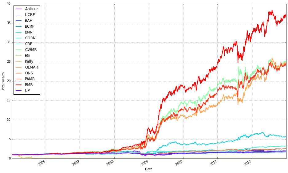
Online Portfolio Selection (OLPS) extends MPT by dynamically updating the assets contained in the selected portfolio by analyzing new data as it is collected [5–6]. There is extensive literature on this subject and several approaches to optimize a portfolio with such names as Passive-Aggressive Reversion Strategy (PAMR), OnLine Moving Average Reversion (OLMAR), Robust Median Reversion (RMR). The term reversion refers to the well-tested idea that a financial asset tends to oscillate, on smaller time scales, around a particular trend and when the deviation is large the asset subsequently tends to return to the mean behavior (return to the mean). One can use this principle to observe large deviations from the mean in a particular asset, relative to other assets in a portfolio, and use this information to buy or sell an asset when estimated to be oversold or overbought under the assumption they will increase or decrease in value (if one wants to short the asset for example). Most of the OLPS algorithms are based on the mean reversion idea but some use trend following, that is the principle that an asset that has been growing in price in the recent past will continue to grow in the near future.
When we analyzed several of these published algorithms we found out that they work well under very artificial conditions like no fees or no slippage.
Other people have done similar analyses [7].
But the general idea and approach of OLPS seemed attractive in particular the concept of continuously adapting to the market as new data is acquired.
At the core of the OLPS method is the idea of creating an optimization metric that can assess the behavior of the stock from past information. Then the algorithm assigns a weight to the stocks in the portfolio (that are selected a priori from a given basket, for example, the stocks in NASDAQ 100) that is proportional to the performance metric, giving a larger weight to the worst-performing stocks if a mean reversing strategy is used or larger weight to the best performing stock if a trend following strategy is used.
We spent almost 2 years continuously improving and extracting the essential features in the OLPS approach and developed our own OLPS algorithms and metrics.
Selecting Best Performer Stock
One of the things we discovered early on is that if one gives a 100 % weight to the stock with the larger weight assigned by OLPS algorithms the cumulative growth of the portfolio improves dramatically. This seems counterintuitive because betting on more stocks seems to be a more optimal approach. But all our testing shows that this win-all approach optimizes final cumulative gains. Therefore most of our algorithms focus on a single stock per investment cycle.
Of course, this strategy also increases the volatility of the returns and possible drawdowns.
The idea to select a portfolio with only one stock seems to be contrary to the MPT principle of diversification in investing.
But because we are holding one stock (selected from a large basket of assets) at the time for only a short period the increased risk is still moderate. Also in a sense, our portfolio is diversified over a longer period of time because we do choose a different asset every day (not all at once).
While most of our algorithms focus on a win-all asset, we can increase the number of stocks selected, if necessary, allowing us to trade-off between the growth of the portfolio and risk .
There are several steps in building our algorithms.
- The first is to choose a relevant trading time scale. While trading cryptocurrencies we used a 5 minutes trading period.
- For stocks, after a lot of experimentation, we decided to operate on a daily time scale. This is a very natural time scale for stocks given the US stock market is opened only a limited amount of hours per day and it opens and closes at the exact time every day. Also trading once a day reduces the slippage impact on the total cumulative gain; our measured slippage is about 0.02 % a day, on average, using a relatively simple execution strategy (we are implementing measures to improve on this).
- We collect data every day at a particular time (we have at the moment algorithms that update at 9:40 am eastern and 10:30 am eastern).
- The algorithms perform their calculations within few seconds and apply their metrics to organize the stocks using proprietary sorting criteria from 1 to 100 in terms of their recent performance (measured on different time scales, from few days to up to a couple of weeks).
The metric and sorting are supposed to be predictive of future gains.
This is illustrated in the following figure:
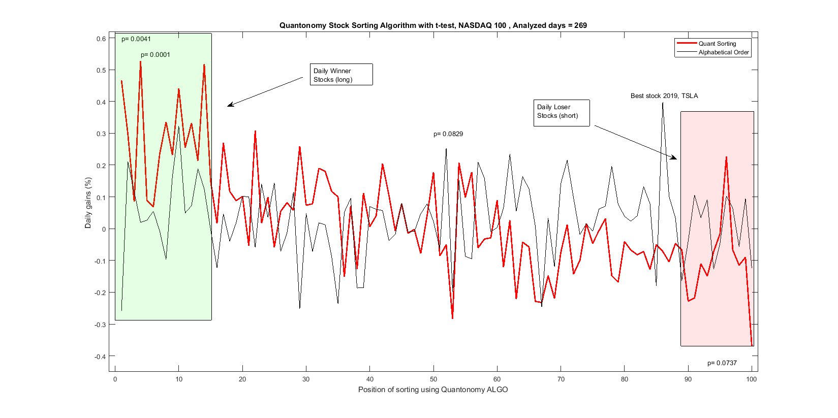
The x-axis shows the position of the stock for a particular day (usually the stock in that position is different every day) from 1 to 100. The position at slot 1 is the position that is supposed to perform best according to the chosen strategy, mean reversion, trend following, or a mix of the two.
The y axis shows the daily gain in percentage averaged over one year. The red curve shows the performance of one of our algorithms. Two areas are highlighted in green and red. The green area shows several positions that seem to outperform the mean behavior of the market (that is mean gain of the 100 stocks over the same period) while the red area shows positions that did relatively worse than average (these stocks can be shorted). The p-values above the data points are obtained through t-tests under the assumption of a Gaussian distribution of the results (that is not exactly correct but a first rough approximation of the true distribution). The p-values do show statistical significance for some of the highest peaks in the red curve. A general overall trend is also observable from the highest values in the green area to the lower values in the red one.
The black curve shows the mean daily averages if we organize the stocks in alphabetical order, that is random. We see that there is not a particular trend. A position seems to be above the others systematically. That is TSLA, Tesla stock that has performed very well over the last year. So in general the market as a whole averages just slightly above zero, while our best sorting position gives us an average gain of 0.5 % per day (for this particular algorithm). That is a return of 250 % in a year.
Walk Forward Optimization
We discussed above the limitation due to overfitting.
A method that is intended to reduce this problem is Walk Forward Optimization [8–9].
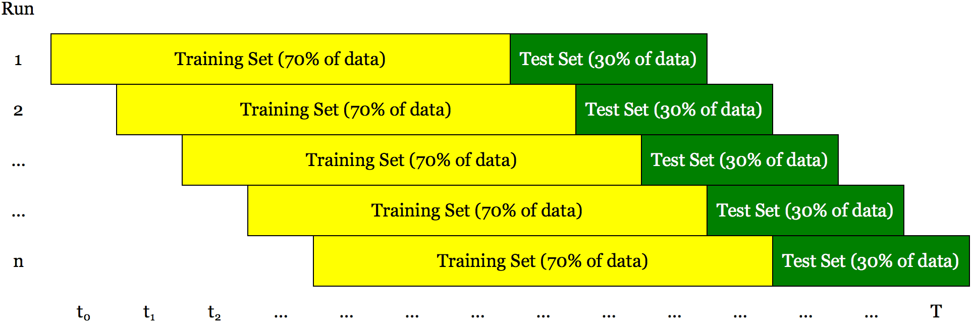
Walk forward optimization is a method used in finance to determine the optimal parameters for a trading strategy. The trading strategy is optimized with in-sample data for a time window in a data series. The remaining data is reserved for out of sampling testing. A small portion of the reserved data following the in-sample data is tested and the results are recorded. The in-sample time window is shifted forward by the period covered by the out-of-sample test, and the process repeated. Lastly, all of the recorded results are used to assess the trading strategy.
The main idea behind walk forward optimization is that to test our algorithms over a training set using a large range of parameters. We can select the parameters that give us the best performances (maximizing a risk measure like Sharpe ratio or final cumulative gain) and assume that what worked in the recent past will hold also for the recent future. As market conditions change we need to retest our strategy and select new parameters that work best for the new conditions.
This approach is both a robustness test and an optimization technique.
It is a robustness test because it can show if the algorithm we are testing can adapt to continuously changing conditions and it is an optimization technique because if the algorithm can adapt then we can find the parameters that optimize its performance in the near future.
Quantonomy adopts walk-forward optimization for all its algorithms.
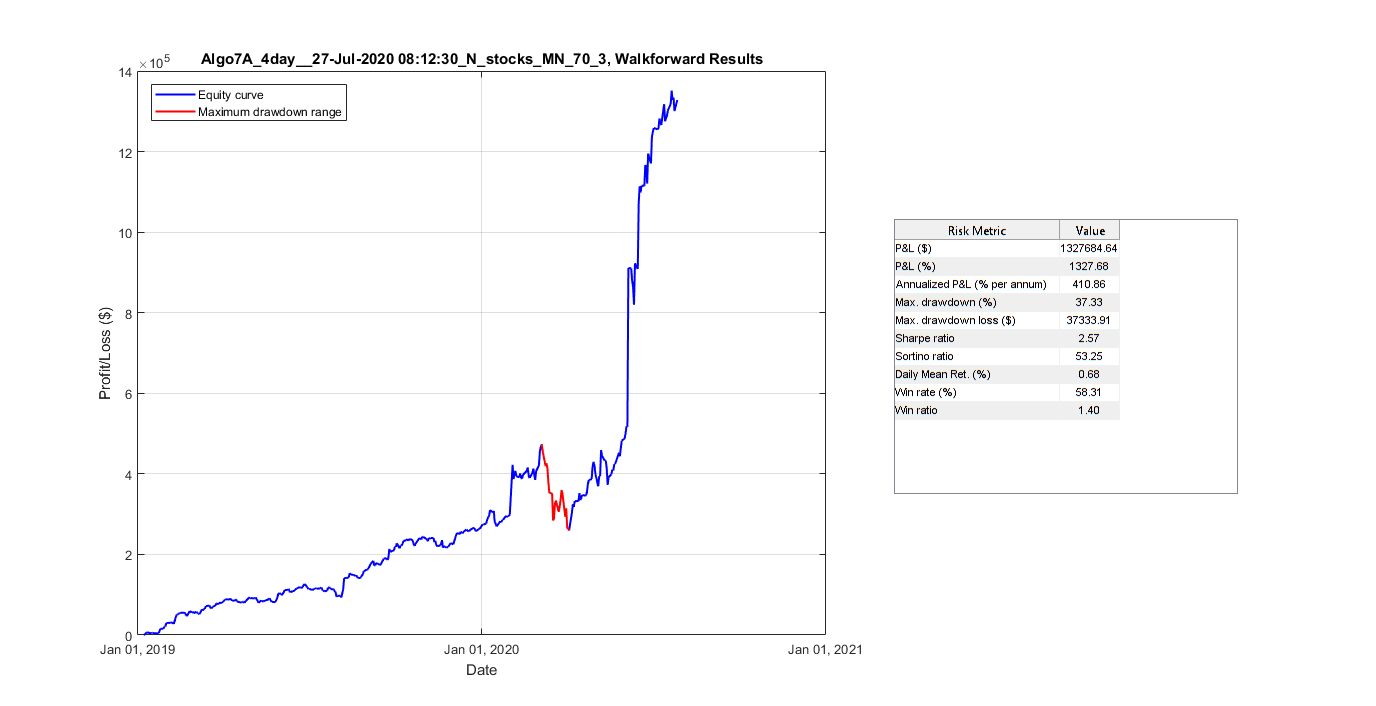
Final cumulative gain graph and statistical results for one of our algorithms after walk-forward testing using third-party software [8].
Statistical Properties of the Algorithms
The profits and losses (PL) of our algorithms may seem completely unpredictable by looking at the cumulative gains chart but actually, they can be fitted by well-known statistical distributions.
There are mathematical tests that can determine the best fitting distribution to the empirical data.
The following picture shows the results of this analysis. The best fit is the tlocationscale distribution.

One of the first things to notice is that this distribution has a heavy tail that means the rare events occur more often than in data with a Gaussian distribution (the typical bell curve distribution). This suggests that relatively large losses or gains can happen relatively often. The distribution is also skewed to the right which means statistically gains are happening more than losses in fact our typical algo wins (returns above 1) about 60 % of the time.
We can then use the theoretical fitted distribution to create a Monte Carlo simulation of the behavior of the trading strategy.
Monte Carlo simulation allows reproducing the statistical behavior of the system represented by certain mathematical distribution thousands of times to analyze the range of possible outcomes when the same experiment is repeated over and over again.
We cannot run our trading strategy over thousands of years in the real world, but a Monte Carlo simulation allows us to do exactly that (even if just virtually). We can then do a statistical analysis of these simulations to infer statistically plausible outcomes of our trading strategy. The following figure shows the results of running the algorithm over 1000 simulations.
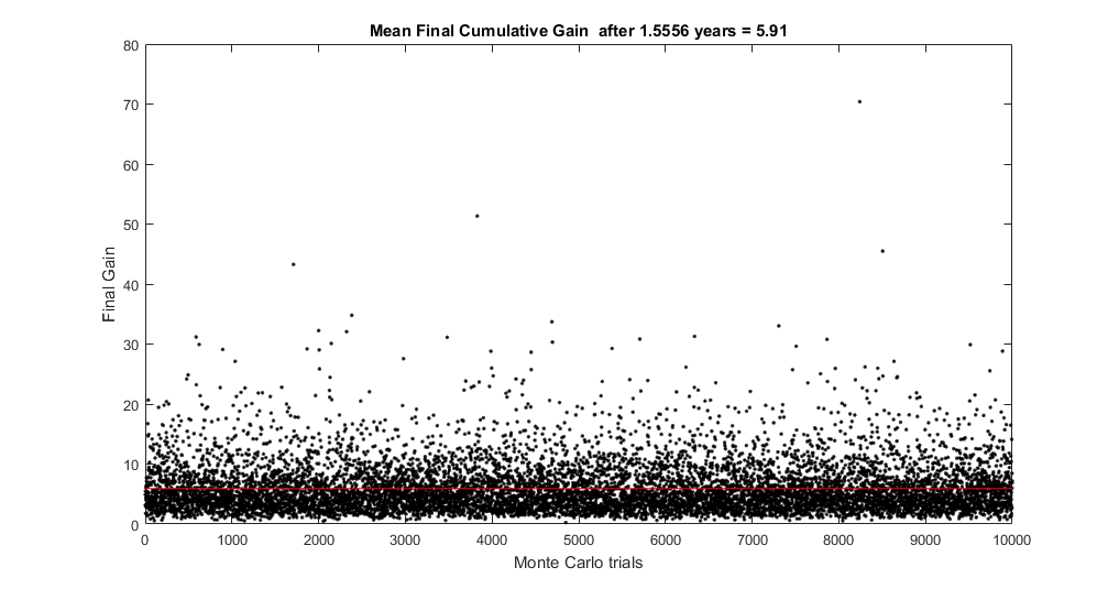
The following figure shows the final gain of these simulations after about 1 and a half years.
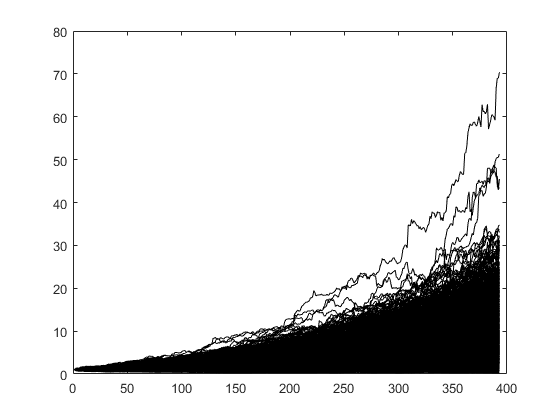
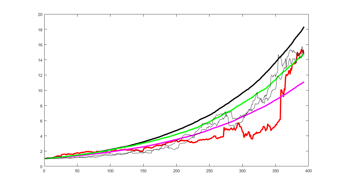
The following figure shows some individual simulations compared with the real behavior of the algorithm (in red). The black line represents a constant return (compounded) of a particular simulation that gave a final cumulative return 1 standard deviation above the mean return of all the 1000 simulations, the purple line is 1 standard deviation below the mean and the green line is a constant return model with a mean return equal to the mean of the entire set of simulations. The purpose of the graph is to show a range of possible likely outcomes (results between the black and purple curves).
The following figure shows the distributions of all final gains of the Monte Carlo simulation.
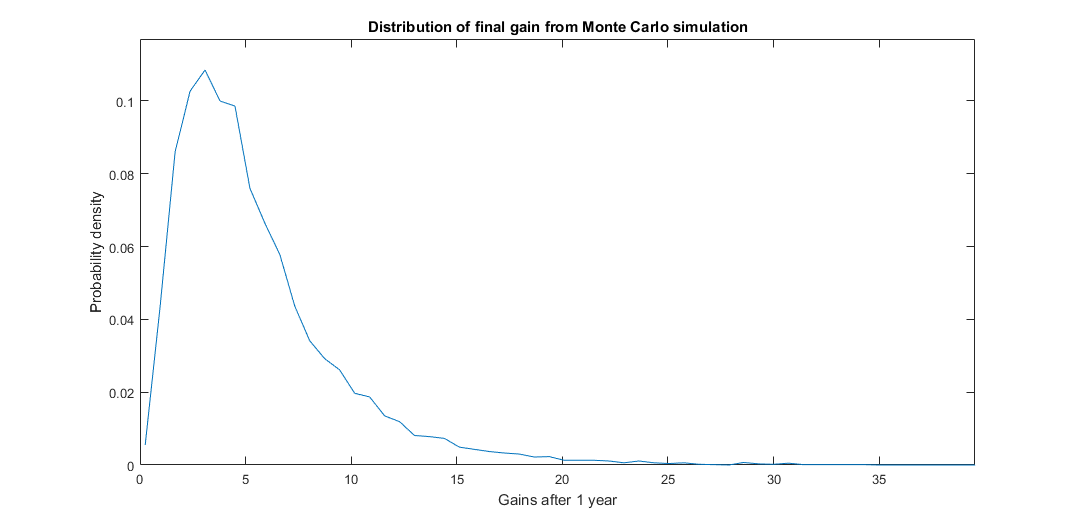
The main conclusion of the Monte Carlo experiment is that after thousands of trials the probability of obtaining a positive PL at all is more than 89 % and the probability of obtaining gains above 2x is about 70 %. The mean gain is 5.91x.
Conclusion
We provided a thorough analysis of a trading strategy including walk forward optimization and the statistical properties of the algorithms. Note for an algorithm to be successful it should be consistent and uncorrelated with market conditions.
Follow us and subscribe at:


References
[1] https://patents.google.com/patent/WO2016028635A1/sv
[2]https://www.reddit.com/r/BitcoinMarkets/comments/29spo8/bitcoin_price_logistic_model/
[3] https://www.nature.com/articles/nphys2648
[4] Markowitz, H.M. (March 1952). “Portfolio Selection”. The Journal of Finance. 7 (1): 77–91. doi:10.2307/2975974. JSTOR 2975974.
[5] Bin L. , Hoi S. C. H. , Online portfolio selection: A survey. https://ink.library.smu.edu.sg/cgi/viewcontent.cgi?article=3263&context=sis_research
[6] https://www.amazon.com/Online-Portfolio-Selection-Principles-Algorithms-ebook/dp/B017K484YM
[7] https://www.quantopian.com/posts/comparing-olps-algorithms-olmar-up-et-al-dot-on-etfs
[8] https://algotrading101.com/learn/walk-forward-optimization/
[9] https://www.youtube.com/watch?v=GNgc0Illar8
[10] https://www.youtube.com/watch?v=OgO1gpXSUzU
Commission-Free trading means that there are no commission charges for Alpaca self-directed individual cash brokerage accounts that trade U.S. listed securities through an API. Relevant SEC and FINRA fees may apply.
Brokerage services are provided by Alpaca Securities LLC ("Alpaca"), memberFINRA/SIPC, a wholly-owned subsidiary of AlpacaDB, Inc. Technology and services are offered by AlpacaDB, Inc.


