I’m a College Student and I Finished Building a Robo Advisor (Part 3)

Hey all, I’m Rao, an intern at Alpaca. This post is the third part in a three-part series. You can find Part 1 and Part 2 on HackerNoon. While those two parts aren’t absolutely necessary to understand this article, I will be making references to topics covered there.

With those two posts, I had built the core of the robo advising process; allocation, distance measuring, and rebalancing. But the allocation process used was hard coded. I found those numbers with an example portfolio online. With modern portfolio theory, all my robo advisor should need is a universe of stocks.

As usual, I did all my work on Quantopian. All you’ll need to replicate my results is a computer and a working internet connection. Let’s get started.

What is Modern Portfolio Theory?

In 1952, Harry Markowitz wrote the paper “Portfolio Selection”. It was groundbreaking and would net him the Nobel Prize for Economics in 1990. In that paper, Markowitz outlined what is now referred to as Modern Portfolio Theory.

Modern Portfolio Theory poses that investors build portfolios that maximize their returns for a given level of risk. The groundbreaking insight was that risk could be evaluated by how they affect the portfolio’s performance, rather than security by security basis.

This meant that investors can construct a set of portfolios that offer the maximum return based on the level of risk.

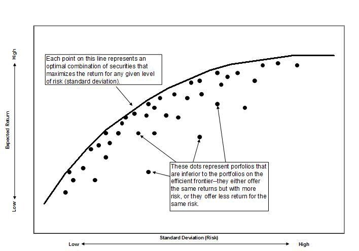
If you’ve read Part 1 or Part 2, you’ll remember that I had a hard-coded risk-based allocation dictionary. With Modern Portfolio Theory, we can calculate that frontier for any universe we have data on.

Implementing MPT in a Robo Advisor

The process of the mean-variance frontier construction will happen in 3 steps:

1. Gather daily returns for the chosen universe
2. Create a mean-variance frontier from the returns given restraints
3. Use basic calculus to find the optimal portfolio

Note that this entire process is allocation. The distance checking and rebalancing portion of the portfolio remains the same. Let’s take a look:

def return_vector(context):
   prices = history(100, '1d', 'price').dropna()
   returns = prices.pct_change().dropna()
    return(returns)def optimal_portfolio(returns):
  n = len(returns)
    returns = np.asmatrix(returns)
     N = 500
    mus = [10**(5.0 * t/N - 1.0) for t in range(N)]
    
    # Convert to cvxopt matrices
  S = opt.matrix(np.cov(returns))
 pbar = opt.matrix(np.mean(returns, axis=1))
    
    # Create constraint matrices
   G = -opt.matrix(np.eye(n))   # negative n x n identity matrix
   h = opt.matrix(-0.15, (n ,1)) #constrains each position to have at least 15% of the available cash. 
        A  = opt.matrix(1.0, (1, n))
    b = opt.matrix(1.0)
    
    # Calculate efficient frontier weights using quadratic programming
    portfolios = [solvers.qp(mu*S, -pbar, G, h, A, b)['x'] 
                  for mu in mus]
    ## CALCULATE RISKS AND RETURNS FOR FRONTIER
    returns = [blas.dot(pbar, x) for x in portfolios]
    risks = [np.sqrt(blas.dot(x, S*x)) for x in portfolios]
   ## CALCULATE THE 2ND DEGREE POLYNOMIAL OF THE FRONTIER CURVE
    m1 = np.polyfit(returns, risks, 2)
    x1 = np.sqrt(m1[2] / m1[0])
    # CALCULATE THE OPTIMAL PORTFOLIO
   wt = solvers.qp(opt.matrix(x1 * S), -pbar, G, h, A, b)['x']
   return np.asarray(wt), returns, risks

The first function return_vector uses Quantopian’s history function to gather daily returns for the last 500 days. It does some minor cleaning and returns the vector s that optimal_portfolio can use it.

Finding the Mean-Variance frontier is an exercise in optimization. Most optimization problems come in a similar format. We have an objective function to optimize. This objective function is often constrained. One example is the fixed equity/income ratio that Vanguard used (from earlier iterations). Constraints are subjective and are a means to have the user essentially set their overarching portfolio preferences.

The objective function is the edge of the Mean-Variance frontier. There are several constraints. The first is that all allocations are between 0 and 1. The second is that the various allocations sum to 1. The last is an optional minimum value for each allocation. In the code above, that’s currently set to 15.

Note: Observe that this value depends on the number of securities in your universe. For example, if your universe has 4 securities, the maximum-minimum allocation (isn’t that a confusing phrase) is 25%.

The second part of the code calculates the 2nd-degree polynomial that represents the edge of all possible portfolios (the frontier) and uses the solver function from the cvx opt package to find the maximum value given the constraints. The weights are returned as a vector to then be individually allocated.

You can play around with the algorithm yourself. Try it here!

Built Robo Advisor

To go ahead and adjust this by yourself, clone the algorithm and go ahead and start editing. To see my thought process, go ahead and check out the medium post regarding this Robo Advisor. Link to come soon!

Rao Vinnakota

Last Thoughts

This article marks the official end of the robo advisor project. I can’t express how much this project has meant to me. It gave me the opportunity to work at Alpaca, jump into a new space, and motivated me to start writing about my experiences.

There are a lot of thank-you’s to go around; to Yoshi, Hitoshi, and the Alpaca team, to Quantopian for the tutorials and the software to experiment, to HackerNoon for publishing my work, and to all the people who reached out to discuss which motivated me to keep working on it. Thank You.

Technology and services are offered by AlpacaDB, Inc. Brokerage services are provided by Alpaca Securities LLC (alpaca.markets), member FINRA/SIPC. Alpaca Securities LLC is a wholly-owned subsidiary of AlpacaDB, Inc.