By Joshua Kyan Aalampour
This content is provided for educational and informational purposes only and should not be construed as investment advice, a recommendation, or an offer to buy or sell any securities or cryptocurrencies. Any strategies, examples, research methodologies, or models discussed are illustrative only and may not be suitable for all investors.
This article reflects the personal experience and opinions of an individual user. Individual experiences will vary, are not representative of all customers, and should not be considered an endorsement or guarantee of future performance. The views expressed are those of the author and do not necessarily reflect the views of Alpaca. Alpaca does not recommend any specific securities or investment strategies. The author was not compensated for this content but did receive nominal promotional items from Alpaca.
Before Quant, There Was Music
My name is Joshua Kyan Aalampour. I’m 24, and most people on the internet know me as a classical composer for piano and orchestra. Quantitative finance came later and I arrived at it through theoretical physics.
As a teenager, I had two real interests: classical music and physics. Music came first. I composed every day. But by the time I was applying to college, I was constantly told the arts had no job stability, so I leaned harder into physics instead. My application essays were about string theory, quantum mechanics, and general relativity. I was accepted to UC Berkeley as a physics student and planned to continue into research and eventually a PhD.
My family did not have money growing up. We moved constantly, spent years motel-hopping, and I missed large parts of high school because of it. Most of my education happened independently through MIT OpenCourseWare lectures, YouTube physics courses, and whatever free resources I could find online.
I eventually won a scholarship that covered two years of tuition. Since I never had much of a social life anyway, I doubled my course load and graduated in half the time.
Then something unexpected happened.
On February 19, 2021, during my freshman year of undergrad, I posted a short video of myself playing my first piano sonata on TikTok. I had no following and no expectations. The video went viral almost immediately. I kept posting, built an audience quickly, and within months music became financially viable enough that I no longer had to worry about survival in the same way.
With money no longer the immediate problem, I returned to physics in my spare time simply because I loved it.
Discovering Quantitative Finance
I got interested in quantitative finance from watching my younger brother. He opened a retail brokerage account, started buying 0DTE options, and experienced a significant gain in a short period, followed by an equally significant loss shortly afterward.
I had no idea what an options contract was or how any of it worked. But his ranting about theta decay and Elon Musk combined with the sheer asymmetry of the bet captured my interest. I felt bad for him, but the fact that this much risk could be opened from a phone was fascinating.
I went down a rabbit hole:
- what an options contract was
- what the Greeks were
- what the Black-Scholes model was
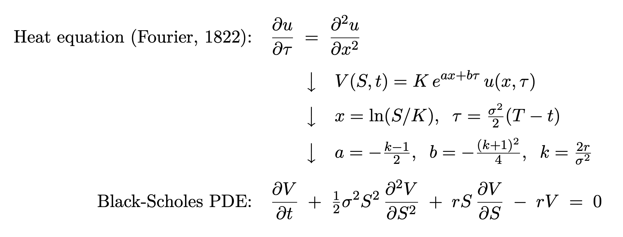
- why Black-Scholes came from the heat equation
For context, the Black-Scholes equation is the Partial Differential Equations (PDE) that prices a European option under no-arbitrage and a log-normal price process. It’s the foundational result in derivatives pricing. Under a change of variables, it actually reduces to the heat equation.
I had read the heat equation a hundred times in physics. Finding it inside a derivative-pricing formula was the first moment I understood that the math I already cared about was the same math the markets used.
It was such a beautiful realization. The substitution absorbs the drift and the discounting:
When Physics and Markets Became the Same Language
From there I started deriving every model I could find from first principles.
Black-Scholes was only the beginning. Its assumptions — constant volatility, continuous paths, log-normal prices — are routinely violated by actual markets, so I moved into more advanced models:
- Merton jump diffusion
- Dupire local volatility
- Heston stochastic volatility
- Bates
- SABR (Stochastic Alpha, Beta, Rho)
- rBergomi (rough Bergomi)
Each model exists because the previous one fails somewhere.
SABR became the one I found most elegant, not because of the model itself, but because of the way I approached deriving it.
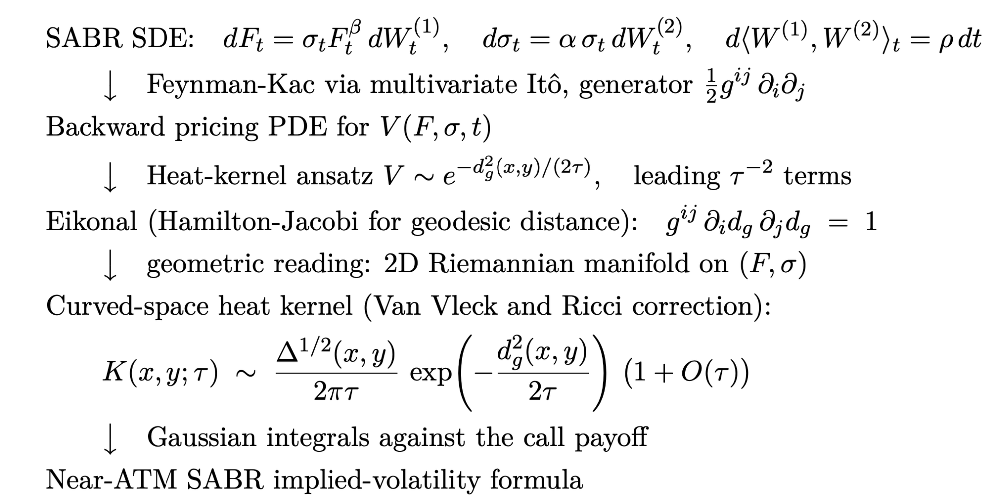
Instead of using the standard perturbation expansion, I took the geometric route. Starting from the stochastic differential equation, I applied Feynman-Kac to obtain the backward pricing PDE, then used a WKB/Laplace ansatz similar to semiclassical methods in quantum mechanics.
The result becomes a Hamilton-Jacobi equation on a two-dimensional Riemannian manifold whose coordinates are the forward price and stochastic volatility.
At that point the problem becomes differential geometry:
- metric tensors
- geodesic distance
- Christoffel symbols
- Ricci curvature
- Laplace-Beltrami operators
- curved-space heat kernels
It was the same mathematical language I had grown up with in general relativity, now appearing inside derivatives pricing.
That realization changed how I viewed quant finance entirely.
Quant as Creative Work
That kind of derivation isn’t engineering to me. The reason I love composing is because I’m actually creating something.
This might sound controversial, but in my opinion, learning to play Chopin’s etudes perfectly doesn’t take creativity. Technical ability? Absolutely. But not creativity. You’re learning to reproduce an existing work.
Composition is creativity.
I think quant finance works the same way.
You can learn to calibrate Heston to a volatility surface or run someone else’s mean-reversion strategy, and that’s honest work, but it’s the same act as performing an existing piece of music.
In my experience, interesting research questions often come from:
- assumptions nobody questioned
- tools from other disciplines nobody thought to apply
- structural identities between fields nobody connected before
To me, quantitative finance feels much closer to artistic creation than people expect.
Building Strategies That Survive Reality
The workflow took me longer to get right than the mathematics.
My earliest backtests overfit badly. Strategies that looked strong historically decayed almost immediately once tested in Alpaca’s paper trading environment.
That experience forced me to rethink evaluation entirely.
I eventually settled on a workflow built around:
- walk-forward validation
- out-of-sample testing
- purged and embargoed cross-validation
- T+1 execution assumptions
Walk-forward testing means training on a rolling historical window, evaluating on the next unseen segment, then repeating the process forward through time.
Traditional k-fold cross-validation assumes samples are independent and identically distributed. Financial returns are neither. Ignoring that tends to inflate Sharpe ratios in proportion to how badly you want the strategy to work.
The purging and embargo methodology comes from Marcos López de Prado’s Advances in Financial Machine Learning. If labels depend on future returns, nearby samples contaminate each other unless explicitly removed.
The embargo is not glamorous, but it matters.
Naive k-fold tends to inflate the score because training labels can have return windows that overlap with the test return windows. Purged k-fold drops those contaminated samples. The gap is a rough measure of the optimism introduced by leakage.
This is a leakage diagnostic, not a production backtest, so the returns are close-to-close, costs are ignored, and the score is not a true Sharpe ratio.
Using Alpaca for Strategy Validation
Alpaca became useful once I started moving beyond pure research into testing and execution.
I use Alpaca’s Market Data to pull daily SPY bars, calculate momentum features, and evaluate strategies under both naïve and purged validation frameworks. The same infrastructure then extends naturally into paper trading for forward evaluation.
What mattered most to me was workflow simplicity.
Instead of building execution infrastructure from scratch, I could:
- pull market data
- run experiments
- validate strategies
- and test live behavior in paper trading
All inside the same environment.
The biggest difference between theoretical research and trading systems is that markets eventually force honesty. Paper trading can help identify differences between research assumptions and observed trading behavior, although paper trading may not fully reflect live market conditions.
Paper trading became the bridge between elegant mathematics and actual operational testing.
from datetime import datetime
import numpy as np
import pandas as pd
from alpaca.data.enums import Adjustment
from alpaca.data.historical import StockHistoricalDataClient
from alpaca.data.requests import StockBarsRequest
from alpaca.data.timeframe import TimeFrame
from sklearn.ensemble import RandomForestClassifier
from sklearn.model_selection import KFold

client = StockHistoricalDataClient("YOUR_KEY", "YOUR_SECRET")
bars = client.get_stock_bars(StockBarsRequest(
    symbol_or_symbols="SPY",
    timeframe=TimeFrame.Day,
    start=datetime(2022, 1, 1),
    end=datetime(2024, 12, 31),
    adjustment=Adjustment.ALL,
))
close = bars.df.xs("SPY", level=0)["close"]

H = 5
LOOKBACK = 20
data = pd.DataFrame({
    "r1":    close.pct_change(1),
    "r5":    close.pct_change(5),
    "r20":   close.pct_change(LOOKBACK),
    "r_fwd": close.pct_change(H).shift(-H),
}).dropna()
X = data[["r1", "r5", "r20"]].values
r = data["r_fwd"].values
y = (r > 0).astype(int)

def oos_score(splits):
    rets = []
    for tr, te in splits:
        m = RandomForestClassifier(max_depth=5, random_state=0)
        m.fit(X[tr], y[tr])
        rets.extend(m.predict(X[te]) * r[te])
    rets = np.array(rets)
    return np.sqrt(252 / H) * rets.mean() / rets.std()

def purged_kfold(n, k, h, e):
    fold = n // k
    for i in range(k):
        a, b = i * fold, (i + 1) * fold if i < k - 1 else n
        keep = np.ones(n, dtype=bool)
        keep[max(0, a - h - e):b + h + e] = False
        yield np.where(keep)[0], np.arange(a, b)

naive = KFold(5, shuffle=False).split(X)
purged = purged_kfold(len(X), 5, max(H, LOOKBACK), 2)

print("Naive  score:", round(oos_score(naive),  2))
print("Purged score:", round(oos_score(purged), 2))
From Research to Execution
For T+1 execution, the signal uses data through the close of day T, and the trade fills at the open of day T+1.
This rules out the most common backtest fictions:
- filling at a price you only knew after the bell
- assuming instantaneous fills at closing prices
- the “4:00 PM order that somehow gets 3:59:59 prices”
My goal is for the equity curve to reflect assumptions that could reasonably have been implemented in practice.
Before any sleeve trades live, it runs through the same execution code path in Alpaca’s paper environment until paper trading results are evaluated against the assumptions used in the backtest.
Alpaca became useful once I started moving from pure research into operational testing:
- pulling historical data
- validating signals
- paper trading strategies
- and testing execution assumptions inside one environment
The markets can eventually force honesty. A strategy either survives contact with reality or it doesn’t.
ORIA: A Multi-Sleeve Quant Architecture
An architecture I’ve been working on is called ORIA: Orthogonal Risk Integrated Alpha.
ORIA is a small multi-sleeve quant book. The goal of the architecture is not to predict markets perfectly, but to combine multiple independent research approaches while managing overlap and risk.
There are currently three research sleeves:
- a directional forecaster built on a compact causal convolutional network
- a relative-value engine built on graph diffusion and topological summaries of cross-sectional residuals
- a small ETF-shock follow-through-or-snapback engine
Above the sleeves sits:
- an orthogonalization layer
- a regime-conditioned allocator
- a risk box with hard caps
- and an execution governor that de-grosses when implementation physics get worse
I won’t go into the specific signals, but the architecture itself I can walk through.
I think the relative-value engine is the most interesting one.
The Relative-Value Engine
The relative-value sleeve treats the active universe as a dynamic graph.
In each session, related names are linked by a nonnegative symmetric similarity matrix W, and a normalized graph Laplacian is built:
L = I - D^{-1/2} W D^{-1/2}
Where D is the diagonal degree matrix.
When the cross-section is shocked by some same-session vector u, the sleeve does not trade u directly. It first computes the graph-smoothed expectation of how that shock should have propagated.

That’s the heat kernel on a graph. The exponential of a Laplacian solves heat conduction in flat continuous space, and a curved-space version of the same construction powered the SABR derivation earlier. Finding the exponential of a Laplacian inside a relative-value sleeve felt the same way as finding the heat equation inside Black-Scholes. The same operators keep showing up in places I don’t expect them!
The signal I study is not the diffused expectation itself, but the residual:
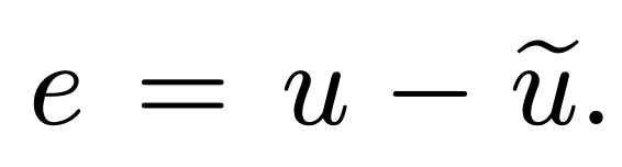
That is the part of the cross-section’s response that the network of relationships did not explain. Topological and distributional summaries of that residual field (connected components, persistence, tail mass, etc.) are one input used when evaluating the residual structure before generating forecasts.
Above the sleeves sits an orthogonalization layer. Three sleeves only help if their risks don’t overlap. If two of them both lean long-market, the book counts the same beta twice. If both end up overweight in tech, then that’s also bad because you’d have too much concentration in one sector. The orthogonalization layer strips this overlap in two stages. First, each raw sleeve is projected onto the common-factor-neutral subspace (market beta, sectors, and styles all get removed) in a risk metric Ω. Second, the factor-cleaned sleeves are symmetrically decorrelated against each other using Löwdin’s construction (originally from quantum chemistry, where it orthonormalizes a basis of atomic orbitals!).
Each sleeve keeps its own intended risk scale. The overlap is theoretically removed when 𝜆= 0. A small shrinkage trades exact orthogonality for numerical stability in practice. There is no hard priority order between sleeves.

The math here is obviously borrowed, but what is mine is the amalgamation: which graph, how
to normalize the Laplacian, how 𝜏 is scheduled, which filtration tells the truth about residual
structure, which factors live in 𝐹, which risk metric Ω, etc., and how all of it producing forecasts intended to account for transaction costs.
What I Learned Building Quant Systems
Some things I’ve learned through developing and testing quantitative trading systems:
Complexity isn’t free
Adding more sleeves, features, and parameters does not always improve the book. Eventually complexity adds noise faster than signal.
Scalability is hard
A strategy that works at $100k may fail at $10M. Liquidity is finite, slippage scales with participation, and alpha decay becomes measurable.
Metrics can mislead
I’ve seen people optimize for the highest Sharpe possible while sacrificing actual returns. Sharpe rewards reducing volatility just as much as growing returns, and the same strategy can produce wildly different Sharpe ratios across regimes.
One number is never enough.
Outside ORIA, I’ve also been writing about a connection between control theory and market microstructure.
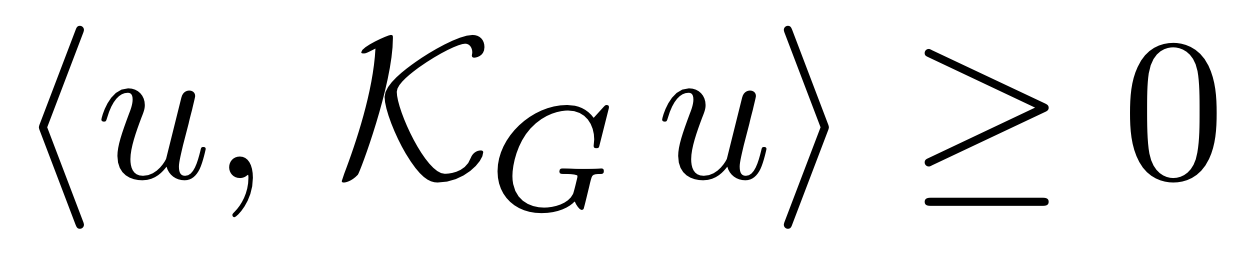
Admissibility of a transient cross-impact kernel turns out to satisfy the same inequality that control theorists call passivity. The two fields identified the condition independently.
It’s probably not implementable on smaller accounts, but the deeper structural connection is what interests me.
What’s Next
Right now I’m continuing to refine both the mathematical and operational sides of my workflow:
- improving validation methods
- experimenting with different volatility structures
- refining execution sensitivity
- and building systematic strategies from first principles
What interests me most is not finding a perfect strategy.
It’s building frameworks that remain intellectually honest under uncertainty.
Markets change constantly. Models fail constantly. The work is learning how to adapt without abandoning rigor.
Additional Alpaca Resources
If you want to start building your own systematic trading system, here are the resources I found most useful:
Alpaca Trading API (docs.alpaca.markets/docs/trading-api) is the place to start. The paper trading quickstart will have you placing simulated orders quickly.
Alpaca Market Data API (docs.alpaca.markets/docs/about-market-data-api) provides the historical and real-time data that powers everything. I found the free tier (IEX feed) is more than enough to get started.
Alpaca Paper Trading (docs.alpaca.markets/docs/paper-trading) lets you set up a paper account in minutes. Same API, same execution.
About the Author
Joshua Kyan Alampour is a classical composer and independent quantitative researcher with a background in physics and mathematical finance. His work focuses on derivatives modeling, systematic trading research, and cross-disciplinary approaches to quantitative finance.
*The Paper Trading API is offered by AlpacaDB, Inc. and does not require real money or permit a user to transact in real securities in the market. Providing use of the Paper Trading API is not an offer or solicitation to buy or sell securities, securities derivative or futures products of any kind, or any type of trading or investment advice, recommendation or strategy, given or in any manner endorsed by AlpacaDB, Inc. or any AlpacaDB, Inc. affiliate and the information made available through the Paper Trading API is not an offer or solicitation of any kind in any jurisdiction where AlpacaDB, Inc. or any AlpacaDB, Inc. affiliate (collectively, “Alpaca”) is not authorized to do business.
Descriptions of quantitative models, validation techniques, backtesting, paper trading, research methodologies, and system architectures are provided solely for educational purposes. Any discussion of these topics is illustrative only and should not be interpreted as evidence that any methodology or strategy will produce profitable trading results or be suitable for any investor. Backtesting and paper trading have inherent limitations and may not accurately reflect actual trading results or live market conditions, including the effects of liquidity, transaction costs, slippage, latency, or investor behavior.
Alpaca and the entities referenced in this article are not affiliated and are not responsible for the liabilities of the others.
Alpaca does not prepare, edit, or endorse Third Party Content. Alpaca does not guarantee the accuracy, timeliness, completeness or usefulness of Third Party Content, and is not responsible or liable for any content, advertising, products, or other materials on or available from third party sites.
All investments involve risk, including the possible loss of principal. Past performance, hypothetical results, and backtested performance do not guarantee future results. There is no guarantee that any investment strategy will achieve its objectives. Diversification does not ensure a profit or protect against loss. Investors should carefully consider their investment objectives and risks before investing.
Options trading is not suitable for all investors due to its inherent high risk, which can potentially result in significant losses. Please read Characteristics and Risks of Standardized Options before investing in options.
Securities brokerage services are provided by Alpaca Securities LLC ("Alpaca Securities"), member FINRA/SIPC, a wholly-owned subsidiary of AlpacaDB, Inc. Technology and services are offered by AlpacaDB, Inc.
This is not an offer, solicitation of an offer, or advice to buy or sell securities or cryptocurrencies or open a brokerage account or cryptocurrency account in any jurisdiction where Alpaca Securities or Alpaca Crypto, respectively, are not registered or licensed, as applicable.