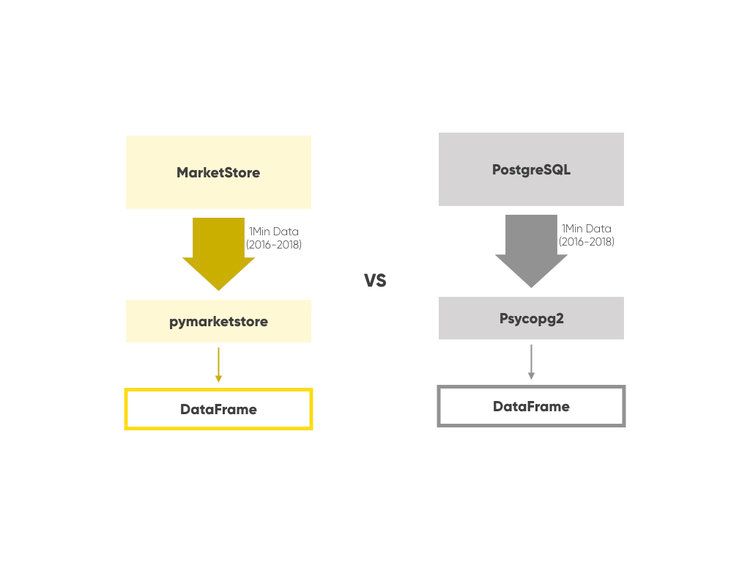
In our last post “How to Setup Bitcoin Historical Price Data for Algo Trading in Five Minutes”, we introduced how to set up bitcoin price data in five minutes and we got a lot of good feedback and contributions to the open source MarketStore.
The data speed is really important
Today, I wanted to tell you how fast MarketStore is using the same data so that you can see the performance benefit of using the awesome open source financial timeseries database.
Faster data means more backtesting and more training in machine learning
Faster data means more backtesting and more training in machine learning for our trading algorithm. We are seeing a number of successful machine learning-based trading algos in the space, but one of the key points we learned is the data speed is really important. It's important not just for backtesting, but also for training AI-style algorithms since it by nature requires an iterative process.
This is another post to walk you through step by step. But TL;DR, it is really fast.
Setup

Last time, we showed how to setup the historical daily bitcoin price data with MarketStore.
This time, we store all the minute-level historical prices using the same mechanism called background worker, but with a slightly different configuration.
root_directory: /project/data/mktsdb
listen_port: 5993()
# timezone: "America/New_York"
log_level: info
queryable: true stop_grace_period: 0
wal_rotate_interval: 5
enable_add: trueenable_remove: false
enable_last_known: false
triggers:
 - module: ondiskagg.so
       on: "*/1Min/OHLCV"
config:
  destinations:
       - 5Min
       - 15Min
       - 1H
       - 1D
bgworkers:
   - module: gdaxfeeder.so
       name: GdaxFetcher
config:
    query_start: "2016-01-01 00:00"
    base_timefame:“1Min”
- BTC
Almost 2.5 years with more than 1 million bars
The difference from last time is that background worker is configured to fetch 1-minute bar data instead of 1-day bar data, starting from 2016-01-01. That is almost 2.5 years with more than 1 million bars. You will need to keep the server up and running for a day or so to fill all the data, since GDAX’s historical price API does not allow you to fetch that many data points quickly.
Again, the data fetch worker carefully controls the data fetch speed in case the API returns “Rate Limit” error. So you just need to sleep on it.
Additional configuration here is something called “on-disk aggregate” trigger. What it does is to aggregate 1-minute bar data for lower resolutions (here 5 minutes, 15 minutes, 1 hour, and 1 day).
Check the longer time horizon to verify the entry/exit signals
In a typical trading strategy, you will need to check the longer time horizon to verify the entry/exit signals even if you are working on the minute level. So it is a pretty important feature. You would need pretty complicated LEFT JOIN query to achieve the same time-windowed aggregate in SQL. But with MarketStore, all you need is this small section in the configuration file.
The machine we are using for this test is a typical Ubuntu virtual machine with 8 of Intel(R) Xeon(R) CPU E5-2673 v3 @ 2.40GHz, 32GB RAM and SSD.
The Benchmark
Unfortunately lots of people in this space are using some sort of SQL database
We are going to have a DataFrame object in python which holds all the minute level historical price data of bitcoin since January of 2016 from the server. We compare MarketStore and PostgreSQL.
PostgreSQL is not really meant to be the data store for this type of data, but unfortunately lots of people in this space are using some sort of SQL database for this purpose since there is no other alternative. That’s why we built MarketStore.
The table definition of the bitcoin data in PostgreSQL side looks like this.
btc=#: prices
         Table "public.prices"
 Column       |              Type                |   Modifiers
----------------+--------------------------------+-------------
   t          |   timestamp without time zone    |
   open       |   double precision               |
   high       |   double precision               |
   low        |   double precision               |
   close      |   double precision               |
   volume     |   double precision               |
The code
# For postgres
def get_df_from_pg_one(conn, symbol):
tbl = f'""'
cur = conn.cursor()
# order by timestamp, so the client doesn’t have to do it
cur.execute (f"SELECT  t, open, high, low, close, volume  FROM ORDER BY  t")
  times   = []
  opens   = []
  highs   = []
  lows    = []
  closes  = []
  volumes = []
for t, open, high, low, close, volume in  cur.fetchall():
     times.append(t)
     opens.append(open)
     highs.append(high)
     lows.append(low)
     closes.append(close)
     volumes.append(volume)

return pd.DataFrame(dict(
   open   = opens
   high   = highs
   low    = lows
   close  = closes
   volume  = volumes
), index=times)
# For MarketStore
def get_df_from_mkts_one(symbol):
params pymkts.Params(symbol, '1Min', 'OHLCV')
return pymkts.Client('http://localhost:6000/rpc').query(params).first().df()
You don’t need much client code to get the DataFrame object
The input and output is basically the same, in that one symbol name is given, query the remote server over the network, and get one DataFrame. One strong benefit of MarketStore is you don’t need much client code to get the DataFrame object since the wire protocol is designed to give an array of numbers efficiently.
The Result
First, PostgreSQL
%time  df = example.get_df_from_pg_one(conn, 'prices')
CPU times:  user 8.11 s, sys: 414 ms, total: 8.53 s, Wall time: 15.3 s
And MarketStore
%time  df = example.get_df_from_mkts_one('BTC')
CPU times: user 109 ms, sys: 69.5 ms, total: 192 ms, Wall time: 291 ms
Both results of course look the same like below.
In [21] df.head()
 Out[21]:
                        open      high      low       close    volume
 2016-01-01 00:00:00    430.35    430.39    430.35    430.39   0.0727
 2016-01-01 00:01:00    430.38    430.40    430.38    430.40   0.9478
 2016-01-01 00:02:00    430.40    430.40    430.40    430.40   1.6334
 2016-01-01 00:03:00    430.39    430.39    430.36    430.36   12.5663
 2016-01-01 00:04:00    430.39    430.39    430.39    430.39   1.9530
50 times difference
A bitcoin was about $430 back then… Anyway, you can see the difference between 0.3 vs 15 seconds which is about 50 times difference. Remember, you may need to get the same data again and again for different kinds of backtesting and optimization as well as ML training.
Also you may want to query not just bitcoins but also other coins, stocks and fiat currencies, since the entire database wouldn’t fit into your main memory usually.
Scalability advantage in MarketStore
MarketStore can serve multiple symbol/timeframe in one query pretty efficiently, whereas with PostgreSQL and other relational databases you will need to query one table at a time, so there is also scalability advantage in MarketStore when you need multiple instruments.
Querying 7.7K symbols for US stocks
To give some sense of this power, here is the result of querying 7.7K symbols for US stocks done as an
%time  df = example.get_dfs_from_pg(symbols)
CPU times:  user 52.9 s, sys:  2.33 s, total: 55.3 s, Wall time: 1min 26s
%time df = example.get_dfs_from_mkts(symbols)
CPU times:  user 814 ms, sys: 313 ms, total: 1.13 s, Wall time: 6.24 s
Again, the amount of data is the same, and in this case each DataFrame is not as large as the bitcoin case, yet the difference to expand to large number of instruments is significant (more than 10 times). You can imagine in real life these two (per instrument and multi-instruments) factors multiply the data cost.
Alpaca has been using MarkStore in our production
Alpaca has been using MarkStore in our production for algo trading use cases both in our proprietary customers and our own purposes. It is actually amazing that this software is available to everyone for free, and we leverage this technology to help our algo trading customers.
Thanks for reading and enjoy algo trading!
