Alternative Bars in Alpaca: Part II- (Analysis & Trading Strategy)

• This article is inspired by the book Advances in Financial Machine Learning.
• This project’s Github Repository: https://github.com/Harkishan-99/Alternative-Bars

In the previous part (Part-I) of this article, we learned the intuition behind “alternative” bars and ways to generate them using Alpaca API. We had also discussed various bar types - tick, volume and dollar bars. In this second part of the article series, we will have an in-depth analysis of these bars along with time bars for comparison and will demonstrate an application of “alternative” bars in a simple (intraday) trading strategy with volume bars, all using the Alpaca API.

Part - I (Introduction): In this part, we will learn to generate various alternative bars especially event-driven bars like tick bars, volume bars and dollar bars.

Generating Alternative Bars in Alpaca (Part 1 - Introduction)

Showing you how to generate various alternative bars especially event-driven bars like tick bars, volume bars and dollar bars

Alpaca ResourcesHarkishan Singh Baniya

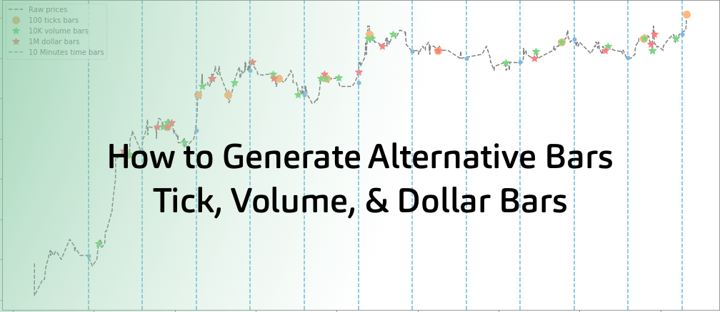
Part - II (Analysis & Trading Strategy): In this part, we will analyze various event-driven bars that were generated in Part-I and will also develop a simple trading strategy using the same bars.

Part - III (Integration in Alpaca API and an ML Trading Strategy): In this part, we will learn to build a live machine learning-based strategy that uses the Alpaca Trade API integration for alternative bars.

Analysis

So in the previous part, I have discussed two major flaws of time bars: assuming markets are chronological by generating bars at a constant time interval and the poor statistical properties that they carry like serial-correlations and non-normality. Now lets understand if “alternative” bars help us mitigate these two flaws and do an in-depth analysis. I have developed an IPython notebook to run these analyses and tests.

Dataset

Before we move on with the test, let’s discuss the dataset used for analysis so that the results are reproducible. I have used AAPL (Apple Inc.) trade data collected from Polygon.io to generate historical alternative bars with historical periods from Jan 1st 2018 to Dec 31st 2019. The trades dataset can be published due to the license agreement, but the bars generated are available in the Github repo of this project. The time bars are the 5-minute bars pulled from Alpaca Data API, also available in the same repo. (*Please do note that this is for illustration only and is not a recommendation or suggestion of this trade or this stock*)

The thresholds used for sampling the bars are:

a) Tick Bars - 5,000 (ticks)

b) Volume Bars - 700,000 (quantity)

c) Dollar Bars - 150,000,000 (dollar)

The thresholds are chosen such that it yields 25-30 bars a day. This is not the ideal way of choosing a threshold in practice, I will discuss a more practical way of choosing a threshold in the later section of the trading strategy.

# read data and store the bars in a dictionary
def read_data(symbol: str):
    path = 'sample_datasets/analysis/'
    bars = {}
    bars['time_bar'] = trim_df(pd.read_csv(path+f'{symbol}_5minute_bars.csv',
                                           index_col=[0], parse_dates=True))
    bars['tick_bar'] = trim_df(pd.read_csv(path+f'{symbol}_tick_bars.csv',
                                           index_col=[0], parse_dates=True))
    bars['volume_bar'] = trim_df(pd.read_csv(path+f'{symbol}_volume_bars.csv',
                                             index_col=[0], parse_dates=True))
    bars['dollar_bar'] = trim_df(pd.read_csv(path+f'{symbol}_dollar_bars.csv',
                                             index_col=[0], parse_dates=True))
    return bars
# trim the after market data if any


def trim_df(df: pd.DataFrame):
    try:
        df = df.tz_localize('UTC').tz_convert('US/Eastern')
    except TypeError as e:
        df = df.tz_convert('US/Eastern')
    idx = df.index
    c1 = (idx.time < dt.time(9, 30))
    c2 = (idx.time > dt.time(16, 0))
    df = df[~(c1 | c2)]
    return df

The above function reads the data as a pandas DataFrame and stores them as the values of a python dictionary with the keys being bar type. The trim_df() function trims the bars to market hours only.

Bars Counts

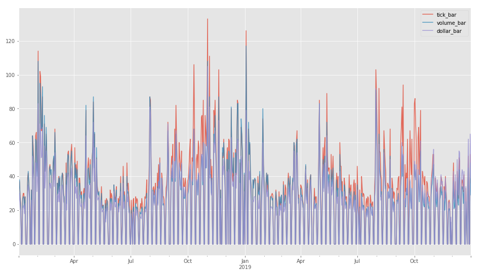
Now let’s see how the intraday bar count looks, this will give us an insight into how stable alternative bars are. In the below figure we see the results of the daily bar count of tick, volume and dollar bars.

Overall bar counts are most stable for dollar bars since they have the least deviation from the mean count, while tick bars have the highest deviation among the three. So, we can expect a more uniform bar generation in case of dollars compared to others.

The above plot was created using a function that groups each of the alternative bars into a group of 1 day using pandas pd.Grouper and counts the number of bars in each daily time group.

# Bar Count Analysis and Plots
def show_bar_count(bars: dict, time_group='1D'):
    counts = {}
    f, ax = plt.subplots(figsize=(16, 9))
    for bar in bars.keys():
        if bar != 'time_bar':
            df = bars[bar]
            count = df.groupby(pd.Grouper(freq=time_group))['close'].count()
            counts[bar] = count
            count.plot(ax=ax, ls='-', label=bar, alpha=0.8)
            print(f'The bar count for {bar} with time group {time_group}\
                  has a mean count of {count.mean()} and a standard deviation
                  of {count.std()}')
    ax.legend()

Also, we also see how different bars are sampled including the time bar for a randomly chosen date from the sample period 2019-08-07 in the above figure. Now from the plot, we can see the uniform time bars, but for the alternative bars we see some clustering at the start and end of the market hours. This was expected as more orders are executed during these periods as a result more information is available. But the time bar was unable to capture it due to its constant sampling frequency.

Normality

Now let’s conduct some statistical tests and look at the statistical properties of the bars. The first test we conduct is a Jarque-Bera test which tests whether sample data have the skewness and kurtosis matching a normal distribution. The statistics we are interested in are the mean, standard deviation, skewness, kurtosis and the most important Jarque-Bera statistics, it will let us know how close the underlying distribution is to the normal distribution.

# Statistical Tests
def get_statistics(bars: dict):
    res = []
    for bar in bars.keys():
        ret = bars[bar].close.pct_change()[1:]
        jb = stats.jarque_bera(ret)[0]
        kurt = stats.kurtosis(ret)
        skew = stats.skew(ret)
        mean = ret.mean()
        std = ret.std()
        res.append([mean, std, skew, kurt, jb])
    return pd.DataFrame(res, index=bars.keys(),
                        columns=['mean', 'std', 'skew',
                                 'kurtosis', 'jarque-bera stats'])

The code above shows a function that takes a dataset dictionary we created above and generates a DataFrame of the statistics mentioned above with index as the bar type.

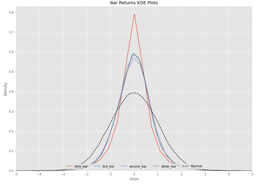
We see the dollar bar has the best statistics among all, especially has the lowest Jarque-Bera stats, skewness and kurtosis. Also, the time bars have the least attractive stats among all. So, the dollar bar is closer to the normal distribution in comparison with other bars followed by the tick and volume bars. Also, in the below figure we see the Kernel Density Estimation (KDE) plot of all the bars along with the normal distribution in black dotted line. Here we see a partial recovery to the normality for the alternative bars (tick, volume and dollar) bars.

Auto-correlation

Finally, let’s look at the auto-correlations of bar returns along with the ACF plot. High auto-correlation can cause model instability and violate model assumptions, especially with Machine Learning models. If you want to know more about why auto-correlations are a problem you can refer to this article.

# ACF Plots
def plot_bar_acf(bars: dict, lags: int = 120):
    fig, axes = plt.subplots(2, 2, figsize=(20, 15))
    loc = [(0, 0), (0, 1), (1, 0), (1, 1)]
    for i, bar in enumerate(bars.keys()):
        ret = bars[bar].close.pct_change()[1:]
        plot_acf(ret, lags=lags, zero=False, ax=axes[loc[i][0], loc[i][1]],
                 title=f'{bar} Auto Correlation with {lags} lag')

The code snippet shows two functions, one to display the auto-correlations of different bars and the other plot the autocorrelation function (ACF) plots. We don’t see any significant auto-correlation at lag=1.

Results

From the above analysis, we can conclude that alternative bars are promising and have attractive properties compared to time bars. But the only factor that affects the bars is its threshold or sampling frequency, a change threshold can bring significant changes in its properties. For analysis, I choose the thresholds arbitrarily, which should not be done if it is applied in practice. A good solution is to use a dynamic threshold (a threshold that keeps changing over time) as a function of a metric that can track market dynamics. Dr de Prado suggested using a function of the free-float market capitalization of stock as a dynamic threshold. A dynamic threshold will be used in the trading strategy we will build. Also, it is not the case that alternative bars always perform better than time bars. Whether to go with a time bar or volume bar or dollar bar depends on the problem we are trying to solve, blindly going with any one of those might lead to a suboptimal result.

Proper statistical tests as shown above and understanding of the bar types should help to choose the right bar for the problem. For example, if we wanted to capture the short-term momentum then we can think using dollar bars and volume bars as the most important factor affecting the short term momentum is trade volume. A second example would explain or capture seasonality in the market, time-bar is a good candidate.

Key Takeaways

• Alternatives bars properties are dependent on the threshold used for sampling.
• Use dynamic threshold while applying alternative bars in practice.
• Choosing the right type of bars depends on the problem we are solving.
• Statistical tests as above helps to choose the right bar for the problem.
• Alternative bars shine well with machine learning models.

Trading Strategy

Now how can a user implement alternative bars in their own strategy? I decided to show an implementation of the realtime streaming alternative bars in a simple intraday trend-following trading strategy. The strategy will be utilizing Bollinger Bands (BB) breakout to generate trading signals. The algorithm doesn’t contain much ‘bells and whistles’ since the aim is not to build a bullet-proof strategy that beats the market. Rather the aim is to show the implementation of alternative bars. An in-depth backtest for the strategy will be shown in the upcoming part of this article series, with ways to improve it further utilizing ML on the alternative bars.

Warning: The following code needs access to Polygon tick data therefore if you do not have a funded live trading account through Alpaca you will receive a Warning Code 1000 followed by an error message of “Invalid Polygon Credentials”.

Rules

• BUY when the closing price crosses the upper BB from below.
• SELL when the closing price crosses the lower BB from above.
• Close a position whenever TP (take profit) or SL (stop-loss) is achieved or a counter position needs to be taken.
• TP and SL decided according to the asset’s volatility.

Bars

I have decided to go with the volume bars with dynamic thresholds that are calculated everyday using an exponentially weighted average of the last 5 days daily traded volume of the asset. The reason for going with the volume bars is that the intraday momentums are greatly influenced by the intraday trading volume, therefore the idea is to capture information of the trend using the traded volume. Another, very good choice would be to use dollar bars using something similar threshold function on the daily market capitalization of that asset.

def on_bar(self, bar: dict):
    """
    This function will be called everytime a new bar is formed. It
    will calculate the entry logic using the Bollinger Bands.

    :param bar : (dict) a Alternative bar generated from 
                EventDrivenBars class.
    """
    if self.collection_mode:
        self.prices = self.prices.append(pd.Series([bar['close']],
                                                   index=[pd.to_datetime(bar['timestamp'])]))
        if len(self.prices) > self.window:
            self.collection_mode = False

    if not self.collection_mode:
        # append the current bar to the prices series
        self.prices = self.prices.append(pd.Series([bar['close']],
                                                   index=[pd.to_datetime(bar['timestamp'])]))
        # get the BB
        UB, MB, LB = ta.BBANDS(self.prices, timeperiod=self.window,
                               nbdevup=2, nbdevdn=2, matype=0)
        # check for entry conditions
        if self.prices[-2] <= UB[-1] and self.prices[-1] > UB[-1]:
            # previous price was at or below the Upper BB and
            # current price is above it.
            self.OMS(BUY=True)
            # GOING LONG
        elif self.prices[-2] >= LB[-1] and self.prices[-1] < LB[-1]:
            # previous price was at or above the Upper BB and
            # current price is below it.
            self.OMS(SELL=True)
            # GOING SHORT

def read_data(self):
    """
    A function to read the historical bar data.
    """
    try:
        df = pd.read_csv(f'data/{self.bar_type}.csv', index_col=[0],
                         parse_dates=[0], usecols=['timestamp', 'symbol', 'close'])
        # the length of minimum data will be the window size +1 of BB
        if not df.empty:
            prices = df[df['symbol'] == self.symbol]['close']
            if len(prices) > self.window:
                self.prices = prices[-self.window+1:]
                del df
                return True

    except FileNotFoundError as e:
        pass

    return False

The above on_bar function will receive a bar generated from the EventDrivenBars class discussed in the previous part. The function then checks if enough historical data is available for calculation of the BB’s using read_data function. If enough data is not available then the algorithm will go into a collection mode and store bars until enough bars are available. An important thing to note here is that the algorithm is not designed to check if the bars are recent, so the user must delete any file that is not updated to recent market data. By the way with enough I mean to say the number of historical bars available must be greater than the window size of the BB’s. If bars are available, then we proceed with calculating the BB’s and check for trading signals and send requests to the OMS (Order Management System) function in case of a trade signal.

Order Management System (OMS) and Risk Management System (RMS)

Now we need to process the trade signals, apply some risk management and send it to the broker. I coded a simple OMS and RMS function to do the task.

def OMS(self, BUY: bool = False, SELL: bool = False):
    """
    An order management system that handles the orders and positions
    for a given asset.
    :param BUY :(bool) If True will buy given quantity of asset at
                market price. If a short sell position is active, it   
                will close the short position.

    :param SELL :(bool) if True will sell given quantity of asset at
                market price. If a long BUY position is active, it will 
                close the long position.
     """
    # check for open position
    self.check_open_position()
    # calculate the current volatility
    vol = self.get_volatility()

    if BUY:
        # check if counter position exists
        if self.active_trade and self.active_trade[0] == 'short':
            # exit the previous short SELL position
            self.liquidate_position()
        # calculate TP and SL for BUY order
        self.tp = self.prices[-1] + (self.prices[-1] * self.TP * vol)
        self.sl = self.prices[-1] - (self.prices[-1] * self.SL * vol)
        side = 'buy'

    if SELL:
        # check if counter position exists
        if self.active_trade and self.active_trade[0] == 'long':
            # exit the previous long BUY position
            self.liquidate_position()
        # calculate TP and SL for SELL order
        self.tp = self.prices[-1] - (self.prices[-1] * self.TP * vol)
        self.sl = self.prices[-1] + (self.prices[-1] * self.SL * vol)
        side = 'sell'

    # check for time till market closing.
    clock = api.get_clock()
    closing = clock.next_close-clock.timestamp
    market_closing = round(closing.seconds/60)

    if market_closing > 30 and (BUY or SELL):
        # no more new trades after 30 mins till market close.

        if self.open_order is not None:
            # cancel any open orders before sending a new order
            self.cancel_orders()
        # submit a simple order.
        self.open_order = api.submit_order(symbol=self.symbol,
                                           qty=self.qty,
                                           side=side, type='market',
                                           time_in_force='day')


def RMS(self, price: float):
    """
    If a position exists than check if take-profit or
    stop-loss is reached. It is a simple risk-management
    function.

    :param price :(float) last trade price.
    """

    self.check_open_position()
    if self.active_trade:
        # check SL  and TP
        if price <= self.sl or price >= self.tp:
            # close the position
            self.liquidate_position()

For any trade signal OMS checks if a counter position exists for a given side and closes the counter position before placing a new order. Before placing a new order we also calculate tp and sl using the get_volatility function. Finally, before placing the order we check if there is enough time left for a new order to capture momentum (30 minute in this case) and also cancel any existing orders on the same security. Since, I am using an older version of Alpaca Python SDK which doesn't support Bracket Order (BO), I had to create a custom RMS to manage the TP/SL as BO. The RMS function is called every time a new trade price is received through the socket, to check TP/SL.

Strategy Instances and Dynamic Thresholds

As during the bar generation process we used several instances for assets so that the algorithm can scale to multi-asset scenario, we will do something similar here. We will assign the assets and strategy settings to instances that receive the responses from the WebSocket streaming API. These instances are reset every day before the market opening with a new threshold for the day calculated using get_current_thresholds function.

def get_current_thresholds(symbol: str, bars_per_day: int, lookback: int):
    """
    Compute the dynamic threshold for a given asset symbol.
    The threshold is computed using exponentially weight average
    of daily volumes for a given decay span. The result is divided
    by 50 to yield approx. 50 bars a day.

    :param symbol : (str) asset symbol.
    :param lookback : (int) lookback window/ span.
    :param bars_per_day : (int) number bars to yield per day.
    """
    df = api.get_barset(symbol, '1D', limit=lookback).df
    thres = df[symbol]['volume'].ewm(span=lookback).mean()[-1]
    return int(thres/bars_per_day)


def get_instances(symbols: dict, bars_per_day: int = 50):
    """
    Generate instances for multiple symbols and configurations for
    the trend trend following strategy.

    :param symbols : (dict) a dictionary with keys as the asset 
                    symbols and values as a list of following - 
                    [bar_type, quantity, window_size, TP, SL] 
                    all in the given order.
    :param bars_per_day : (int) number bars to yield per day.
    """
    instances = {}
    # directory to save the bars
    save_to = 'data'
    for symbol in symbols.keys():
        # create a seperate instance for each symbols
        # thresholds are generated as last 5 days exponential weighted avg. / 50.
        # why 50 ?? to  yield approx. 50 bars a day.
        bar_type = symbols[symbol][0]
        qty = symbols[symbol][1]
        TP = symbols[symbol][3]
        SL = symbols[symbol][4]
        window = symbols[symbol][2]
        # create objects of both the classes
        instances[symbol] = [EventDrivenBars(bar_type,
                                             get_current_thresholds(symbol, bars_per_day,
                                                                    lookback=5), save_to),
                             TrendFollowing(symbol, bar_type, TP, SL,
                                            qty, window)]

    return instances

We iterate through each asset and assign an instance of EventDrivenBars and the TrendFollowing class as a dictionary value. For threshold values, we call get_current_thresholds function to get the dynamic threshold that is set fixed with a lookback value of 5 days, i.e. it will take the last 5 days exponential average and divide it by 50 (for the strategy). Why 50? Because the idea is to yield 50 volume bars a day.

def run(assets: dict, bars_per_day: int = 50):
    """
    The main function that run the strategy.

    :param assets : (dict) a dictionary with keys as the asset symbols and
                    values as a list of following - [bar_type, quantity,
                    window_size, TP, SL] all in the given order.

    :param bars_per_day : (int) number bars to yield per day.
    """
    # a variable that signifies if the strategy is running or not
    STRATEGY_ON = True
    clock = api.get_clock()
    if clock.is_open:
        pass
    else:
        time_to_open = clock.next_open - clock.timestamp
        print(f"Market is closed now going to sleep for \
               {time_to_open.total_seconds()//60} minutes")
        sleep(time_to_open.total_seconds())

    # close any open positions or orders
    close_all()

    channels = ['trade_updates'] + ['T.'+sym.upper() for sym in
                                    assets.keys()]

    # generate instances
    instances = get_instances(assets, bars_per_day)

    @conn.on(r'T$')
    async def on_trade(conn, channel, data):
        if data.symbol in instances and data.price > 0 and data.size > 0:
            bar = instances[data.symbol][0].aggregate_bar(data)
            instances[data.symbol][1].RMS(data.price)  # check TP & SL
            if bar:
                instances[data.symbol][1].on_bar(bar)

    conn.run(channels)

    while True:
        clock = api.get_clock()
        closing = clock.next_close-clock.timestamp
        market_closing = round(closing.seconds/60)

        if market_closing < 10 and STRATEGY_ON:
            # liquidate all positions at 10 mins to market close.
            close_all()
            STRATEGY_ON = False

        if not clock.is_open:
            # keep collecting bars till the end of the market hours
            next_market_open = clock.next_open-clock.timestamp
            sleep(next_market_open.total_seconds())
            # resetting the thresholds and created new instances
            instances = get_instances(assets)
            STRATEGY_ON = True

Now to run the algorithm and start the streaming data we will use the run function as shown in the above code snippet. First, it checks if the market is open, then it generates the instances. We handle the incoming trade data using the aggregate_bar function of EventDrivenBars class and when a bar is generated it is passed to the on_bar function of the strategy. Before, 10 minutes to market closing we liquidate all the positions and set the algorithm to sleep until the next market opens.

Conclusion

In this part, I have shown an analysis of “alternative” bars and how to implement them in a trading strategy. Again, the goal of this article was not to develop a strategy that profits consistently. In the upcoming part, we will see a backtest analysis of this strategy and try to improve it using a machine learning technique called meta labelling and meta-model (to know more, refer to page 50 of AFML).

See also

Using Bollinger Bands to Gauge Trends

Learn three Bollinger Bands® strategies that can be used for analysis or generating trade signals.

InvestopediaCory Mitchell

BlackArbsCEO/Adv_Fin_ML_Exercises

Experimental solutions to selected exercises from the book [Advances in Financial Machine Learning by Marcos Lopez De Prado] - BlackArbsCEO/Adv_Fin_ML_Exercises

GitHubBlackArbsCEO

https://mlfinlab.readthedocs.io/en/latest/implementations/data_structures.html

Technology and services are offered by AlpacaDB, Inc. Brokerage services are provided by Alpaca Securities LLC (alpaca.markets), member FINRA/SIPC. Alpaca Securities LLC is a wholly-owned subsidiary of AlpacaDB, Inc.

You can find us @AlpacaHQ, if you use twitter.