Alternative Bars in Alpaca: Part III - (Machine Learning Trading Strategy)

This article is inspired by the book Advances in Financial Machine Learning.

In the previous part (part-II) of this article, we created a simple (intraday) trading strategy with volume bars, using the Alpaca API. In this last part of the series on alternative bars, we will discuss meta-labelling, a way to filter out the false positives of the trading strategy. Then we will train an ML (meta-model) on those labels to predict whether to act on or pass a trade and compare that with the normal versions of the strategy. It is highly recommended to read the previous parts of the articles to get a better context.

Part - I (Introduction): In this part, we will learn to generate various alternative bars especially event-driven bars like tick bars, volume bars, and dollar bars.

Generating Alternative Bars in Alpaca (Part 1 - Introduction)

Showing you how to generate various alternative bars especially event-driven bars like tick bars, volume bars and dollar bars

Alpaca ResourcesHarkishan Singh Baniya

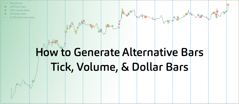
Part - II (Analysis & Trading Strategy): In this part, we will analyze various event-driven bars that were generated in Part-I and will also develop a simple trading strategy using the same bars.

Alternative Bars in Alpaca: Part - II (Analysis & Trading Strategy)

We will analyze various event-driven bars and will develop a simple trading strategy using the same bars.

Alpaca ResourcesHarkishan Singh Baniya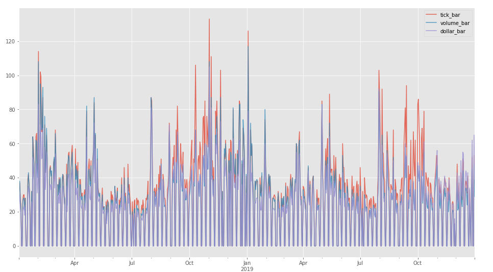

Part - III (A ML Trading Strategy): In this part, we will learn to build a live machine learning-based strategy implementing the alternative bars.

The IPython notebook for this article can be found on the Github repo of this project below.

Harkishan-99/Alternative-Bars

Generate various Alternative Bars both historically and at real-time. - Harkishan-99/Alternative-Bars

GitHubHarkishan-99

Intuition behind Meta-Labelling

In an intuitive level meta-labelling is the process of labelling historical bets whether they were profitable or not. A meta-model can further be trained using these labels to identify the false-positives from a trading strategy or a model and avoid those trades. The idea of meta-labelling was introduced in the book Advances in Financial Machine Learning (page-50 3.6) and the author suggested that meta-labelling can be used to learn the bet size of the primary prediction model. Since it is a binary classification problem of whether to trade or not to trade, it presents a trade-off between type-I errors (false positives) and type-II errors (false negatives). So, our goal is to reduce the false positives but by doing that we tend to reduce the true positives, which ultimately reduces the number of trades taken. Therefore, the trade-offs need to be dealt with accordingly and by the end of this article, we shall learn to do that.

We will be using the meta-labels to generate a meta-model that can identify whether we should act or pass on the signals given the Bollinger Bands trading strategy. The algorithm for meta-modelling is neatly packed in the mlfinlab python package which I will be using. To better understand the meta-labelling in-depth and how the algorithm works I recommend reading this article.

Getting the Meta-Labels

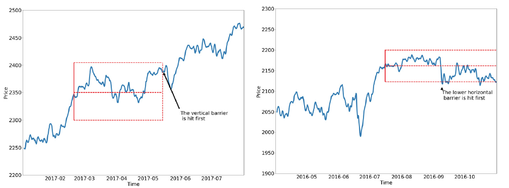
Before getting the meta-labels, let’s understand the get_events function of mlfinlab that we will be using and especially the function parameters. The function uses the triple-barrier method to calculate the returns from a bet. In short, it considers three barriers: the upper and the lower barrier which is set at a distance for the opening price of the bet according to a target (in our case hourly volatility), which is considered as the TP/SL (SL/TP) in meta-labelling for Long (Short) position. And the vertical barrier defines how long a bet stays active i.e. we close the bet if neither TP nor SL is hit (in our case it would be the time when we need to take a counter position). We find which barrier is touched first and calculate the return of the bet till that point; if it’s profitable we label it as 1 else 0.

The most important parameter we will require is the sides generated by our trading strategy. So, I have built a custom function get_sides that identifies the up-cross and the down-cross of the price from the Bollinger bands and outputs a series with sides of the bets and indexed by the timestamps.

def get_sides(df):
    """
    A function to get the trade sides either long
    or short from up or down cross of the price
    from the Bollinger Bands according to the 
    strategy.
    """
    # up-cross
    c1U = df.close.shift(1) < df.UB.shift(1)
    c2U = df.close > df.UB
    # down-cross
    c1D = df.close.shift(1) > df.LB.shift(1)
    c2D = df.close < df.LB
    # signals
    sides = pd.Series(np.nan, index=df.index)
    # LONG
    sides.loc[(c1U) & (c2U)] = int(1)
    # SHORT
    sides.loc[(c1D) & (c2D)] = int(-1)
    return sides.dropna()

We also need the hourly volatility of the bar's closing price which will be used to define the stop-loss (SL) and take-profit (TP) of a bet. The below function gets the hourly volatility with exponential weighting and a user-defined decay span. To know more about Pandas ewm function, you can visit the official documentation.

def get_hourly_volatility(close, lookback=10):
    """
    Get the hourly volatility of a price series with
    a given decay span.
    """
    timedelta = pd.Timedelta('1 hours')
    df0 = close.index.searchsorted(close.index - timedelta)
    df0 = df0[df0 > 0]
    df0 = (pd.Series(close.index[df0 - 1],
                     index=close.index[close.shape[0] - df0.shape[0]:]))
    # hourly returns
    df0 = close.loc[df0.index] / close.loc[df0.array].array - 1
    df0 = df0.ewm(span=lookback).std()
    return df0

As discussed above, we also need a vertical barrier which will be the timestamp where we close the position to take a counter position. The below function loops over the sides taken from the get_sides and finds the point where the sides flip.

def get_vertical_barrier(close, sides):
    """
    This function outputs the timestamps where the
    position is closed due to a counter position that
    had to be taken due to side flip while holding a
    opposite position than the current one. 

    This timestamp will be considered as the vertical
    barrier or the point where we close the position 
    when neither the TP nor the SL hit has occurred.
    """
    # get the positions where side flips
    t1 = pd.Series(pd.NaT, index=close.index)
    prev_side = sides[0]
    last_update = close.index[0]
    for i in range(1, len(sides)):
        if (sides[i] + prev_side) == 0:
            # switch position i.e. close the current position
            # and take a counter position
            t1[last_update:sides.index[i]] = sides.index[i]
            last_update = sides.index[i]
        prev_side = sides[i]
    t1 = t1.fillna(close.index[-1])
    return t1

The get_returns passes all the above parameters along with the user-defined TP and SL multiple for the strategy to the get_events and outputs the first touch. Finally, we return the returns of each bet calculated using get_bins and the side of the bet from get_sides.

def get_returns(bars, tpsl):
    """
    A function to get the strategy returns from the 
    entry sides, volatility and the exit conditions 
    according to the strategy, the get_events function
    from mlfinlab get the returns by applying these 
    parameters.

    :param bars :(pd.DataFrame) bars dataframe.
    :param tpsl :(list) TP and SL for the strategy.

    :return : (pd.DataFrame) a dataframe of the sides
             generated by the strategy and the returns
             for those.
    """
    # signals i.e. LONG/SHORT (1/-1)
    sides = get_sides(bars)
    # hourly volatility
    vol = get_hourly_volatility(bars.close)
    # vertical barrier
    t1 = get_vertical_barrier(bars.close, sides)
    # get the 3B events
    triple_barrier_events = ml.labeling.get_events(close=bars['close'],
                                                   t_events=sides.index,
                                                   pt_sl=tpsl,
                                                   target=vol,
                                                   min_ret=0.0,
                                                   num_threads=4,
                                                   vertical_barrier_times=t1,
                                                   side_prediction=sides)
    labels = ml.labeling.get_bins(triple_barrier_events, bars['close'])
    return labels[['ret', 'side']]

Modelling

For the modelling, I have used a random forest classifier model that is fed with a feature set and the meta-labels and this will be our meta-model. Since we have only talked about the labels let's discuss the features and the preprocessing steps. I have done some feature engineering and added the returns, volatility, momentum (5 periods) and RSI (5 periods) of the closing price. These are some features that I believe are relevant to a trend following strategy. One must invest more time doing this kind of feature engineering and add more relevant features for developing a robust model. For the training itself, I have separated an out-of-sample dataset for validation and getting the returns performance metrics. The train_model function fits the classifier and prints the out-of-sample scores, confusion matrix and returns the predictions.

def train_model(X, y, split_date):
    """
    A function to train a Random Forest as meta model 
    on the given features(X) and labels(y) and return 
    the prediction for out-of-sample (OOS) validation.
    """
    X_train, y_train, X_val, y_val = X[:split_date], y[:split_date],
    X[split_date:], y[split_date:]
    # defining a random forest model
    model = RandomForestClassifier(n_estimators=800, max_depth=7,
                                   criterion='entropy', random_state=1,
                                   n_jobs=-1)
    # fitting the model
    model.fit(X_train, y_train)
    # OOS prediction
    y_pred = model.predict(X_val)
    # displaying models performance metrics out-of-sample (OOS)
    print(f'(OOS) Accuracy : {accuracy_score(y_val, y_pred)}')
    print(f'(OOS) Precision : {precision_score(y_val, y_pred)}')
    print(f'(OOS) Recall : {recall_score(y_val, y_pred)}')
    print(f'(OOS) Confusion Matrix : \n {confusion_matrix(y_val, y_pred)}')
    return y_pred

Analysis

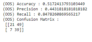
Okay, a lot of work has been done, let’s see if all of this has any meaningful effect on our strategy. To understand how I ran the analysis and the report, I request the reader to view the IPython notebook for this article. If we look at the out-of-sample (OOS) performance of the model itself we can see that it didn’t do much well in terms of accuracy and precision but has a good recall score (as shown below). It was somewhat expected as I didn’t put much effort into the model through hyper-parameter tuning, feature selection, or adding more features. In a real investing application of this model, one is expected to use large sets of features and refine the selection using feature selection techniques.

Now let’s check the trading performance of the plain strategy returns vs the strategy with the meta-model working on top as a trade signals filter. The returns are the output from get_bins and are trimmed to match the OOS dataset index. The meta-model signals are binary so they are multiplied to the plain strategy returns. So, does it perform any better? Well, below is the performance report (generated by pyfolio) for both.

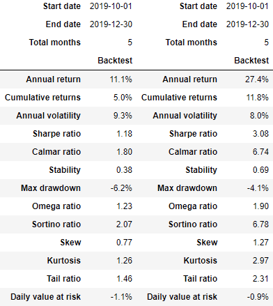
Comparing the above reports we see a significant improvement of the meta-model strategy in all the key performance metrics like the Sharpe ratio that has increased from 1.18 to 3.08, the max drawdown has improved from -6.2% to -4.1%, the annual volatility has decreased from 9.3% to 8.0% and the cumulative return has increased from 5.0% to 11.8%. So, overall we can say that the meta-model has good work in filtering out the false positives of the strategy.

Conclusion

To conclude, this article series I would like to say that alternative bars are promising especially in machine learning mainly due to their better statistical properties and event-driven nature. This was empirically proven in the first two parts of the article series. Then, we created a simple trend-following strategy using volume bars, a common type of alternative bars. Finally in this part, we have learnt to create a meta-model on top of the existing strategy to maximize the potentials of the volume bars. Though the model performance metrics like accuracy and precision were not that great, we have achieved a significant performance increase with the meta-model. The meta-model helped to reduce the max drawdown and increase the overall Sharpe ratio, which was expected, as the main motive was to filter out as many false positives as possible. A risk-averse investor can trade some of the recall from the model to increase the precision by keeping a threshold on the predicted probability of accepting a trade (e.g. at 60%) from the meta-model. This way the investor can reduce their max drawdown and volatility further, but it may sacrifice some potential returns due to the decrease in the number of trades.

To apply this meta-model in the live trade setting, I would recommend the following steps to improve the robustness of the model.

• Use more relevant features for training.
• Do features selection and feature engineering.
• Tune the hyper-parameters of the model with cross-validation.
• For the testing, I would recommend using an online learning setup for the model training and testing with a moving window to keep the model relevant with the new information to avoid rapid decay in performance.

Currently, the integration of alternative bars into an official plugin repository is in progress and will be released at an undetermined later date. Once the repository is released a short follow-up article will be published noting the additional steps needed to implement alternative bars into a strategy. For now, thank you for following this article series, and please reach out if you have any questions.

References

To understand this article better I recommend you the following resources and also the book mentioned above:

Using Bollinger Bands to Gauge Trends

Learn three Bollinger Bands® strategies that can be used for analysis or generating trade signals.

InvestopediaCory Mitchell

• https://github.com/Hudson-and-Thames-Clients/research/blob/master/Advances%20in%20Financial%20Machine%20Learning/Labelling/BBand-Question.ipynb
• https://mlfinlab.readthedocs.io/en/latest/labeling/tb_meta_labeling.html
• http://www.epchan.com/Meta-labelling.pdf

Technology and services are offered by AlpacaDB, Inc. Brokerage services are provided by Alpaca Securities LLC (alpaca.markets), member FINRA/SIPC. Alpaca Securities LLC is a wholly-owned subsidiary of AlpacaDB, Inc.

You can find us @AlpacaHQ, if you use twitter.