2021 has been a torrential year for Bitcoin. Its violent movements this year have been driven primarily by changes in the global regulation and adoption of cryptocurrencies. Bitcoin’s large presence in financial markets and dramatic movements seems to have increased many peoples investment interest in it.
Although Bitcoin may boast large returns, simply buying and holding Bitcoin can be a nail biting prospect. Its volatility can induce portfolio drawdowns large enough to make most investors question whether they should sell. An alternate strategy to simply buying and holding volatile assets like Bitcoin, is to follow the trend; that is, buy only when there is a bullish trend and sell when that trend comes to an end. A simple way to help achieve this is by looking at the crossovers of simple moving averages (SMA). SMAs allow us to “smooth” out the price data and make trends more easily identifiable.
SMAs of different periods can help us identify trends. When a short period SMA crosses over a long period SMA, it may signal a change towards a more bullish trend. We can look to buy when such a crossover happens and sell when the short period SMA crosses under the long period SMA, potentially signalling the end of the trend.
We can evaluate whether such a strategy would perform well by performing a backtest. There are many open source backtesting libraries available, but for this example, we will take a more vanilla approach. We will use only pandas to backtest our strategy and Plotly to chart our results.
Alpaca’s Market Data API can be a powerful tool for easily accessing market data. Since Alpaca recently launched Cryptocurrency trading and market data, we can also access crypto data from the same API. We can use the Market Data API to access all the equity and crypto data we will need for our backtest.
Crypto and Equity Data with Alpaca’s Market Data API
Getting Started
In order to perform our backtest, we will need to retrieve historical data for SPY* and Bitcoin over 2021. The Market Data API allows us to easily access both equity and cryptocurrency data.
Before we get started, we will need to import some libraries that we will be using.
The alpaca-trade-api will allow us to access market data for Bitcoin and SPY. We will use Bitcoin data to conduct our backtest and SPY data to determine its relative performance. We will also use pandas for data manipulations and backtesting. Finally, Plotly will let us make beautiful charts to display our results.
# Alpaca for data
import alpaca_trade_api as api
from alpaca_trade_api.rest import TimeFrame

# pandas for analysis
import pandas as pd

# Plotly for charting
import plotly.graph_objects as go
import plotly.express as px

# Set default charting for pandas to plotly
pd.options.plotting.backend = "plotly"
Setting the Backtest Configurations
As mentioned in the beginning of the article, we want to test how our strategy would have performed during 2021. We’ll take a look at daily data for both BTCUSD and SPY between January 1st 2021 and October 20th 2021.
# symbols we will be looking at
btc = "BTCUSD"
spy = "SPY"

# start dates and end dates for backtest
start_date = "2021-01-01"
end_date = "2021-10-20"

# time frame for backtests
timeframe = TimeFrame.Day
For our simple moving average (SMA) crossover strategy, we’ll be using 2 SMAs of different daily periods. We will use a pair that is commonly used: the 5 day SMA with the 13 day SMA.
# periods for our SMA's
SMA_fast_period = 5
SMA_slow_period = 13
Accessing Alpaca Market Data
We can access both stock and crypto data with the Market Data API. We simply have to create an instance of the Alpaca API with our credentials. If you don’t know where to find your credentials, you can learn about it in this article.
Now, we can make a request to the API for daily bar data between our selected dates. Make a note of the different syntax between crypto and equity data.
# Our API keys for Alpaca
API_KEY = "YOUR_ALPACA_API_KEY"
API_SECRET = "YOUR_ALPACA_API_SECRET"
# Setup instance of alpaca api
alpaca = api.REST(API_KEY, API_SECRET)
# # # Request historical bar data for SPY and BTC using Alpaca Data API
# for equities, use .get_bars
spy_data = alpaca.get_bars(spy, timeframe, start_date, end_date).df
# for crypto, use .get_crypto_bars, from multiple exchanges
btc_data = alpaca.get_crypto_bars(btc, timeframe, start_date, end_date).df
# display crypto bar data
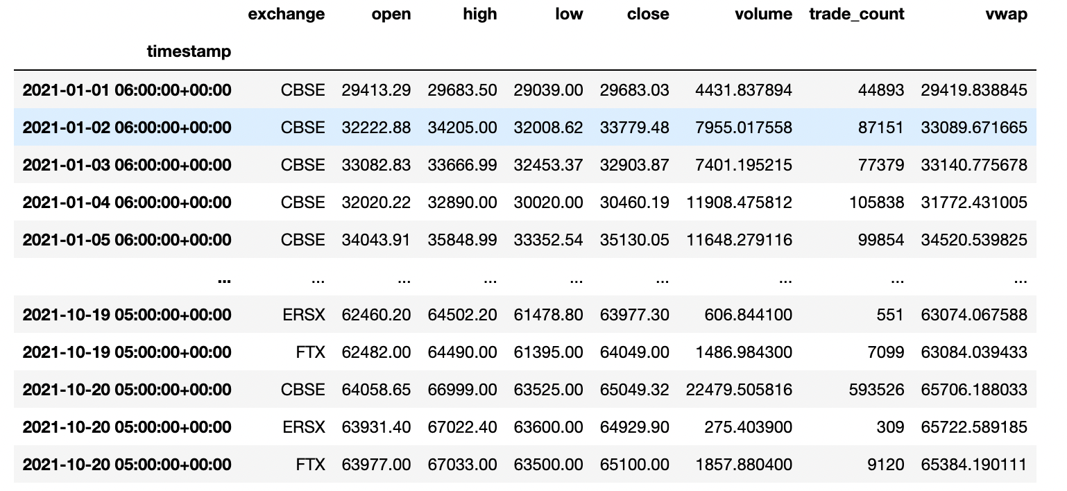
btc_dataThe market data for Bitcoin is stored as a dataframe. Look at the figure below to see how it is structured. The raw data from the API has many different fields, including open, high, low, close (OHLC), volume (in number of coins), trade_count and volume weighted average price (vwap) and finally the exchange that the data is from.
Keep in mind, there may be duplicate data for the same timestamp from different exchanges in the raw data. We can see this with ‘ERSX’ and ‘FTX’ near the bottom of the dataframe.
Bitcoin vs SPY During 2021
Cleaning and Organizing Our Market Data
Our API call returned many different fields, however we only need the daily closing price for our backtest. This means we can drop all columns except the ‘close’ column. To make it easier to distinguish between BTC and SPY, we’ll rename our close field to their respective symbols. We also can keep just the date part of our timestamp, this will make it easier to relate BTC prices to SPY prices. Finally, for BTC, there is duplicate data from multiple exchanges, let’s use data just for a single exchange: ‘CBSE’.
# Keep data from only CBSE exchange
btc_data = btc_data[btc_data['exchange'] == 'CBSE']

# keep only the daily close data column
btc_data = btc_data.filter(['close'])

# rename our close column to BTC
btc_data.rename(columns={'close':'BTC'}, inplace=True)

# keep only the date part of our timestamp index
btc_data.index = btc_data.index.map(lambda timestamp : timestamp.date)

# Clean SPY data
spy_data = spy_data.filter(['close'])
spy_data.rename(columns={'close':'SPY'}, inplace=True)
spy_data.index = spy_data.index.map(lambda timestamp : timestamp.date)
Now we can combine our two dataframes into one containing both SPY and BTC data. Let’s set our index name to ‘date’ and forward fill any missing data points.
data = btc_data.join(spy_data, how='outer')
data.index.name = 'date'
data = data.ffill()
Bitcoin vs SPY in 2021
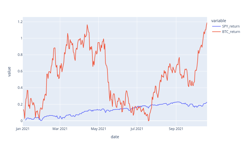
Now that we have our data pampered and ready. There are some interesting things we can look at, such as a comparison of the performance of BTC and SPY. We can calculate the daily returns by using .pct_change(), which will compute the percent difference between each daily close. Then we can calculate a cumulative return by taking the cumulative product of (1 + daily return). We subtract by one to measure our percent return (i.e. 1.54 return is 0.54 or 54%).
# calculate data returns for BTC and SPY
data['SPY_daily_return'] = data['SPY'].pct_change()
data['BTC_daily_return'] = data['BTC'].pct_change()

data['SPY_return'] = data['SPY_daily_return'].add(1).cumprod().sub(1)
data['BTC_return'] = data['BTC_daily_return'].add(1).cumprod().sub(1)

px.line(data,x=data.index, y=['SPY_return', 'BTC_return'])
Finally, let’s plot the cumulative return for BTC and SPY using Plotly.
Computing Simple Moving Average Crossovers
Calculating Simple Moving Averages In Pandas
To test our SMA crossover strategy, we will need to first compute the SMA over our fast and short periods, as defined in previous sections. This is easy to do with pandas, simple moving averages are essentially rolling means. Let’s remove any null data points that may appear and plot BTC’s price with its 5 and 13 day SMAs.
# Computing the 5-day SMA and 13-day SMA
data['slow_SMA'] = data['BTC'].rolling(slow_period).mean()
data['fast_SMA'] = data['BTC'].rolling(fast_period).mean()

data.dropna(inplace=True)

data.plot(y=['BTC', 'slow_SMA', 'fast_SMA'])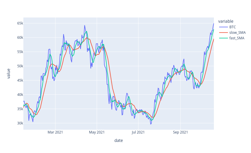
Calculating SMA Crossovers
We can see from the previous chart that the moving averages closely follow the price of BTC. In addition, with careful observation, we can also note that when the fast SMA (green) crosses above the slow SMA (red), BTC’s price lunges upwards. We might also notice that the fast SMA crosses under the slow SMA once the trend begins to reverse. Let’s try to take advantage of this by identifying crossovers and placing trades at those points.
We can create 2 new data frames that will hold precisely when these crossovers and crossunders happen. We can compute a crossover/crossunder by comparing a row to the previous row. For example, if the fast SMA is above the slow SMA in the current row, while in the previous row it is below the slow SMA, a crossover has occurred.
We can use the .shift() method to shift data by 1 row, allowing us to view the past row with the present row.
# calculating when 5-day SMA crosses over 13-day SMA
crossover = data[(data['fast_SMA'] > data['slow_SMA']) \
       & (data['fast_SMA'].shift() < data['slow_SMA'].shift())]

# calculating when 5-day SMA crosses unsw 13-day SMA
crossunder = data[(data['fast_SMA'] < data['slow_SMA']) \
        & (data['fast_SMA'].shift() > data['slow_SMA'].shift())]
Let’s plot our BTC and SMAs as before. But this time we will also plot our crossovers and crossunders as green and red arrows, respectively. Now we can see all the entries and exits our strategy makes during the backtest period.
# Plot green upward facing triangles at crossovers
fig1 = px.scatter(crossover, x=crossover.index, y='slow_SMA', \
                  color_discrete_sequence=['green'], symbol_sequence=[49])

# Plot red downward facing triangles at crossunders
fig2 = px.scatter(crossunder, x=crossunder.index, y='fast_SMA', \
                  color_discrete_sequence=['red'], symbol_sequence=[50])

# Plot slow sma, fast sma and price
fig3 = data.plot(y=['BTC', 'fast_SMA', 'slow_SMA'])

fig4 = go.Figure(data=fig1.data + fig2.data + fig3.data)
fig4.update_traces(marker={'size': 13})
fig4.show()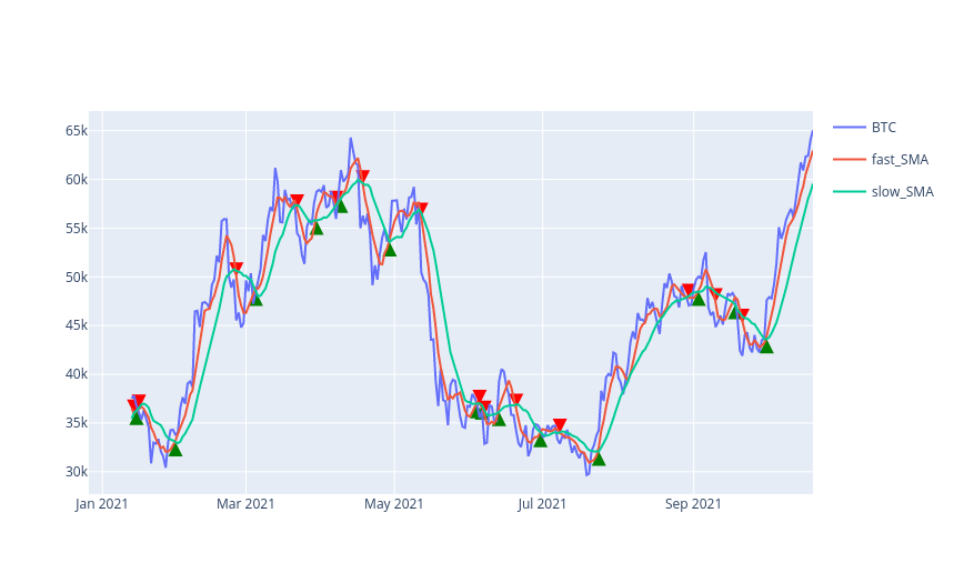
Computing The Backtest and Strategy Performance
Keeping Track Of Orders
We want to translate our crossovers/crossunders into orders during our backtest. Let’s create a new column in our data frames for orders: If on a given row, we want to submit an order, we will have a value of ‘buy’ or ‘sell’, and if there aren’t any orders to be submitted, we will leave it blank (NaN).
We can achieve this by first creating the columns in our crossover and crossunder dataframes and then merging them with our original dataframe. This new merged data frame called portfolio will contain all our market data and the orders we desire. We will use this portfolio data frame to compute our backtest.
# New column for orders
crossover['order'] = 'buy'
crossunder['order'] = 'sell'


# Combine buys and sells into 1 data frame
orders = pd.concat([crossover[['BTC', 'order']], crossunder[['BTC','order']]]).sort_index()

# new dataframe with market data and orders merged
portfolio = pd.merge(data, orders, how='outer', left_index=True, right_index=True)
Computing The Backtest
Everything is now ready for us to begin backtesting. To kick things off, we’ll compute a backtest on how $10,000 would have grown if we bought and held SPY and did the same for BTC, separately. Doing this will help us properly assess our SMA crossover performance.
The buy and hold backtests are simple. We just need to multiply the cumulative returns of each asset with our starting portfolio value $10,000.
# "backtest" of our buy and hold strategies
portfolio['SPY_buy_&_hold'] = (portfolio['SPY_return'] + 1) * 10000
portfolio['BTC_buy_&_hold'] = (portfolio['BTC_return'] + 1) * 10000
Let’s forward fill any missing data. This will smooth the charts we plan to create. We also forward fill the BTC_daily_return because we will be using it for our next backtest.
# forward fill any missing data points in our buy & hold strategies
# and forward fill BTC_daily_return for missing data points
portfolio[['BTC_buy_&_hold', 'SPY_buy_&_hold', 'BTC_daily_return',]] = \
                    portfolio[['BTC_buy_&_hold', 'SPY_buy_&_hold', 'BTC_daily_return']].ffill()
Now, let’s compute, row by row, our portfolio value if we had deployed our SMA crossover strategy during 2021. We will initialize our equity to 10,000 and no active positions.
Then, iterating over each row in our dataframe, if we encounter a “buy”, we set our active position flag to True and if we encounter a “sell”, we set our active position flag to False. This will help us identify when we are invested in BTC, i.e. our portfolio equity’s returns match BTC’s returns.
We’ll store the series of portfolio equity values in a new column called BTC_SMA_crossover. Storing this data will help us create our chart.
### Backtest of SMA crossover strategy
active_position = False
equity = 10000

# Iterate row by row of our historical data
for index, row in portfolio.iterrows():

    # change state of position
    if row['order'] == 'buy':
        active_position = True
    elif row['order'] == 'sell':
        active_position = False

    # update strategy equity
    if active_position:
        portfolio.loc[index, 'BTC_SMA_crossover'] = (row['BTC_daily_return'] + 1) * equity
        equity = portfolio.loc[index, 'BTC_SMA_crossover']
    else:
        portfolio.loc[index, 'BTC_SMA_crossover'] = equity
Let’s plot our three backtests using Plotly and see what the results look like.
fig=px.line(portfolio[['BTC_SMA_crossover', 'BTC_buy_&_hold', \ 'SPY_buy_&_hold']], color_discrete_sequence=['green','blue', 'red'])

fig.show()
The results show that using an SMA crossover performs better than buying and holding BTC. The strategy helps avoid many of the drawdowns.
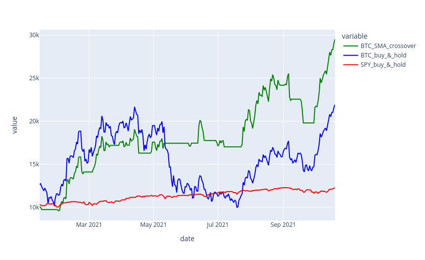
Calculating The Sharpe Ratio
To put our strategy’s performance into perspective, we can calculate its sharpe ratio. Since we do not have a full year’s worth of data, we can calculate the daily sharpe ratio and then annualize it by multiplying it by the square root of the number of trading days in a year. Following through with the calculations below, we see that our strategy produces a Sharpe Ratio of 1.9 during the period.
portfolio['BTC_SMA_daily_returns'] = portfolio['BTC_SMA_crossover'].pct_change()

mean_daily_return = portfolio['BTC_SMA_daily_returns'].mean()
std_daily_return = portfolio['BTC_SMA_daily_returns'].std()
spy_mean_daily_return = portfolio['SPY_daily_return'].mean()

trading_days = 252

daily_sharpe_ratio = (mean_daily_return - spy_mean_daily_return) / std_daily_return

annualized_sharpe_ratio = daily_sharpe_ratio * (trading_days ** 0.5)
annualized_sharpe_ratio
Conclusion
We’ve shown how you can use just data and pandas manipulations to calculate a backtest. Although using a backtesting library can make development easier, they aren’t always necessary. All you need is some good data and creativity. The Market Data API is a powerful tool for better data modelling and backtesting. As cryptocurrencies take off in investment popularity, Alpaca can help provide a seamless environment for both crypto and equities.
*SPY, also known as SPDR S&P 500 Trust ETF (SPY ETF), aims to track the Standard & Poor's 500 Index, which comprises 500 large- and mid-cap U.S. stocks.
Please note that this article is for informational purposes only. The example above is for illustrative purposes only. Actual crypto prices may vary depending on the market price at that particular time. Alpaca Crypto LLC does not recommend any specific cryptocurrencies.
Cryptocurrency is highly speculative in nature, involves a high degree of risks, such as volatile market price swings, market manipulation, flash crashes, and cybersecurity risks. Cryptocurrency is not regulated or is lightly regulated in most countries. Cryptocurrency trading can lead to large, immediate and permanent loss of financial value. You should have appropriate knowledge and experience before engaging in cryptocurrency trading. For additional information please click here.
Cryptocurrency services are made available by Alpaca Crypto LLC ("Alpaca Crypto"), a FinCEN registered money services business (NMLS # 2160858), and a wholly-owned subsidiary of AlpacaDB, Inc. Alpaca Crypto is not a member of SIPC or FINRA. Cryptocurrencies are not stocks and your cryptocurrency investments are not protected by either FDIC or SIPC. Please see the Disclosure Library for more information.
This is not an offer, solicitation of an offer, or advice to buy or sell cryptocurrencies, or open a cryptocurrency account in any jurisdiction where Alpaca Crypto is not registered or licensed, as applicable.