
As markets toss and tumble, many opportunities for trades can be created, and there are a variety of strategies that can be employed. Among these strategies is a special class called market neutral strategies. Market neutral strategies aim to profit regardless of the broader market’s trend.
Market neutral strategies accomplish this by taking simultaneous long and short positions. A common example of a market neutral strategy is to take 50% long and 50% short positions among stocks within a sector, like the technology sector. By doing this, if the sector as a whole plummets, our shorts may increase in value and may help limit our losses. Likewise, if the sector launches upwards, our shorts may decrease in value, which may limit our profits. This feature is what makes this strategy “market neutral”.
In the following sections, we’ll look at historical data to analyze a type of market neutral trade called a pairs trade. Then we will use our analysis of market data to formulate a trading strategy across crypto and equity markets. The Trade API will help us to seamlessly trade cryptocurrencies and equities from the same brokerage account.
What is Pairs Trading?
Pairs trading is an example of a market neutral strategy. Pairs trading attempts to find two highly correlated assets, and take simultaneous long and short positions when their prices deviate, betting that their prices will converge in the future. An example of two such assets can be Bitcoin and Coinbase stock (NASDAQ: COIN), whose prices may be correlated at times due to Coinbase's large crypto balance sheet, and its association with cryptocurrencies.
Getting Started
Let’s compare the minutely returns of Bitcoin and COIN over September 2021. We can use our analysis of this historical data to understand pairs trading and formulate a trading strategy.
There are some libraries we will need to import. We’ll use the alpaca-trade-api SDK to grab historical data, stream live data and place trades and Plotly to chart data. We can then use our API keys to access Alpaca’s APIs. If you want to follow along and place paper trades, make sure to use your paper account’s API Keys.
# Alpaca for data
import alpaca_trade_api as tradeapi
from alpaca_trade_api.rest import TimeFrame

import plotly.graph_objects as go
import plotly.express as px
# Our API keys for Alpaca
API_KEY = "YOUR_API_KEY"
API_SECRET = "YOUR_API_SECRET"

# Setup instance of alpaca api
alpaca = tradeapi.REST(API_KEY, API_SECRET)
Next let’s retrieve minute frame historical data over the 3 month period between August 2021 and November 2021. We will use this data to study the past behavior of COIN and Bitcoin. Since Bitcoin and COIN have dramatically different prices (As of 11/09/21, Bitcoin is at $67,089.48 and COIN is at $357.39). It is better to compare their relative returns rather than their prices. With the historical data, let’s compute the minutely return of each asset and then their cumulative returns.
# Retrieve historical minute data for Bitcoin and Coinbase stock between August 1st 2021 and November 1st 2021
btc = alpaca.get_crypto_bars("BTCUSD", TimeFrame.Minute, "2021-08-01", "2021-11-01").df
btc = btc[btc['exchange'] == 'CBSE']

coin = alpaca.get_bars("COIN", TimeFrame.Minute, "2021-08-01","2021-11-01").df


# minutely return is the percent change of minute price
btc['BTC_minutely_return'] = btc['close'].pct_change()
coin['COIN_minutely_return'] = coin['close'].pct_change()


# cumulative return is the product of each minutely return
# (1 + return_1) * (1 + return_2) * …
btc['BTC_return'] = btc['BTC_daily_return'].add(1).cumprod().sub(1)
coin['COIN_return'] = coin['COIN_daily_return'].add(1).cumprod().sub(1)
If we plot the cumulative returns of the two assets, we may begin to see a pattern emerge. Notice that the returns of Bitcoin and Coinbase seem to closely follow each other, and when the returns do diverge, they tend to realign in the future.
fig1 = px.line(btc, y='BTC_return', color_discrete_sequence=['red'])
fig2 = px.line(coin, y='COIN_return', color_discrete_sequence=['blue'])
fig3 = go.Figure(data=fig1.data + fig2.data)
fig3.show()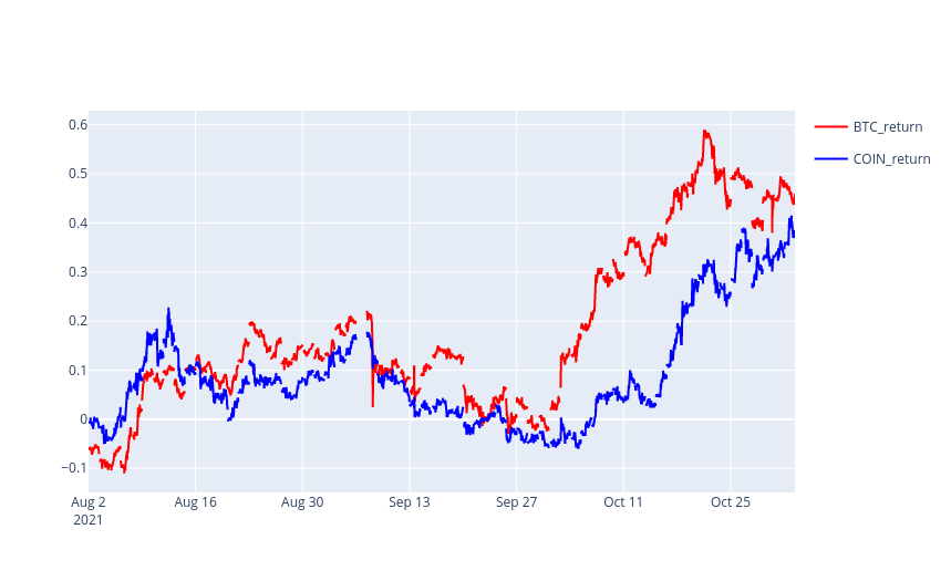
What is a Spread?
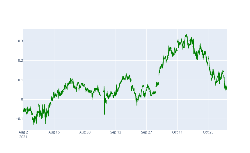
We saw how the returns of Bitcoin and Coinbase seem to be correlated, and when their returns diverge, they seem to converge again in the future. We can make this behavior more noticeable by looking at the spread of the returns. Let’s take a look at BTC_return - COIN_return.
# calculating the spread which is the difference of returns
data['spread'] = data['BTC_return'] - data['COIN_return']

fig1 = px.line(data, y='spread',  color_discrete_sequence=['green'], render_mode='svg')

# Configuring the x-axis to hide weekends. We will be doing this often going forward.
fig1.update_xaxes(
    rangebreaks=[
        { 'pattern': 'day of week', 'bounds': [6, 1]},
        { 'pattern': 'hour', 'bounds':[23,11]}
    ])

fig1.show()
When the spread is 0, the return of Bitcoin and Coinbase are equal. When the spread is greater than 0, the return of Bitcoin is greater than Coinbase and vice versa for a spread less than 0. Notice how the spread seems to eventually revert towards 0 each time the spread’s magnitude increases. If we make the assumption that this pattern will continue, an opportunity for a trade can arise each time the spread deviates from 0.
Formulating a Trading Strategy
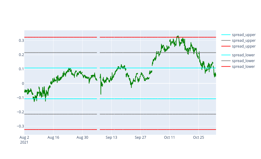
In order to define our strategy well, we will need to be able to measure our spread. One way to measure how large the spread is is to compare the spread to its historical standard deviation. This is better than using just the absolute value of the spread because the standard deviation gives us context of how large the spread is compared to its historical values. Let’s calculate the historical standard deviation over those 3 months. The spread_upper_std is 1 STD above 0 spread and spread_lower_std is 1 STD below 0 spread.
# calculating standard deviation of spread values
historical_spread_std = data['spread'].std()

# defining new column for the standard deviation
data['spread_std'] = historical_spread_std

# defining new columns for positive and negative multiple of the standard deviation, we will use these columns for charting
data['spread_upper_std'] = 1 * data['spread_std']
data['spread_lower_std'] = -1 * data['spread_std']
Let's also plot the different multiples of our standard deviation to see which multiples are most relevant for our strategy. We'll plot the -3, -2, -1, +1, +2, +3 multiples of the STD.
# Plotting 1 multiplied with positive and negative STD in cyan
fig2 = px.line(data * 1, y=['spread_upper_std', 'spread_lower_std'], color_discrete_sequence=['cyan'], render_mode='svg')

# Plotting 2 multiplied with positive and negative STD in gray
fig3 = px.line(data * 2, y=['spread_upper_std', 'spread_lower_std'], color_discrete_sequence=['gray'], render_mode='svg')

# Plotting 3 multiplied with positive and negative STD in red
fig4 = px.line(data * 3, y=['spread_upper_std', 'spread_lower_std'], color_discrete_sequence=['red'], render_mode='svg')

# chart configurations
fig5 = go.Figure(data=fig1.data + fig2.data + fig3.data + fig4.data)
fig5.update_xaxes(
    rangebreaks=[
        { 'pattern': 'day of week', 'bounds': [6, 1]},
        { 'pattern': 'hour', 'bounds':[23,11]}
    ])

fig5.show()
By applying some rudimentary analysis on the chart below, we can see that when the spread leaves the +/-1 STD area marked by the cyan lines, it seems to return into that area in the future. Let’s take advantage of this by placing entry trades whenever the spread crosses the +/- 1 STD spread line. We may exit when the spread returns back to 0 and if the spread continues to increase, we may consider exiting at +/- 3 STD.
Our entry trades will vary on whether the spread has crossed below the -1 STD line or above the +1 STD line. If it is below -1 STD, this means the return of Bitcoin is lower than that of Coinbase. If we want to bet that the spread will close, we can go long on Bitcoin and short Coinbase. This will keep our strategy market neutral.
However, our strategy is limited. According to our analysis, the appropriate trade when the spread crosses above the +1 STD line, should be to short Bitcoin and go long on Coinbase. But because we cannot short Bitcoin, we cannot take advantage of when the spread crosses above the +1 STD line. We are limited to trading on only one side of the spread.
Streaming Live Data via Market Data API
Accessing Live Data
Now that we’ve completed our analysis with historical data, let’s move on to a live data environment and eventually deploy our strategy on to live paper trading. The Market Data API gives us access to live data from both equity and crypto markets. We can do this easily with the SDK by creating an instance of the Stream class and subscribing to data for our desired assets.
The data is delivered to the handler functions on_crypto_bar and on_equity_bar that we defined and passed in as parameters to the subscription methods. The bar data for each subscription will be passed into the handler through the bar parameter each time data is available. In addition, since Bitcoin is traded on multiple exchanges, we want to keep our algorithm simple and avoid duplicate data by looking at bar data from only a single exchange CBSE.
Make a note of the different syntax between equity and crypto data subscriptions. Finally, we can call run to start our data streaming.
# instance of data streaming API
alpaca_stream = Stream(API_KEY, API_SECRET)


# handler for receiving bar data for Bitcoin
async def on_crypto_bar(bar):
    if bar.exchange != 'CBSE':
        return

   print(bar)

# handler for receiving bar data for Coinbase stock
async def on_equity_bar(bar):
    print(bar)


# subscribe to coinbase stock data and assign handler
alpaca_stream.subscribe_bars(on_equity_bar, "COIN")


# subscribe to Bitcoin data and assign handler
alpaca_stream.subscribe_crypto_bars(on_crypto_bar, "BTCUSD")


# start streaming of data
alpaca_stream.run()
For now we are just printing our bar data as it arrives. However, If we run the code above you’ll see that the crypto and equity bars arrive at slightly different times. This happens because the data streams are independent of each other and the data is arriving from different exchanges. This can be a problem for our strategy because our strategy relies on both crypto and equity data being available at the same time so that we can calculate our spread.
Synchronizing Data Streams
We need both equity data and crypto data at the same time before we can start computing the necessary calculations for our strategy. This means if crypto data arrives before equity data, we will need to wait until the equity data arrives before starting. One way we can synchronize our data streams is by collecting our bars into an intermediary data structure before passing the data to our strategy calculations.
Let’s first change our data handlers to pass on their bar data into our intermediary function, that we will call synch_datafeed. In this function that we will soon define, we will synchronize our data feeds so that we can easily access both Bitcoin and COIN bars for the latest timestamp.
# change handlers

async def on_equity_bar(bar):
   # bar data passed to intermediary function
   synch_datafeed(bar)

async def on_crypto_bar(bar):
   if bar.exchange != 'CBSE':
       return
   # bar data passed to intermediary function
   synch_datafeed(bar)
First let’s define a nested dictionary called data, that will hold our crypto and equity data, keyed by the timestamps and symbols of the bars. Let’s also define our function sync_datafeed, which will synchronize our data by timestamp, and then will feed bar data of the latest timestamp to the strategy by passing the data into on_synch_data. Within on_synch_data we can access data for COIN and Bitcoin when they both become available.
 # Define dictionary to organize our data
data = {}

def synch_datafeed(bar):
   # convert bar timestamp to human readable form
   time = datetime.fromtimestamp(bar.timestamp / 1000000000)
   symbol = bar.symbol

   # If we’ve never seen this timestamp before
   if time not in data:
       # Store bar data in a dictionary keyed by symbol and wait for data from the other symbol
       data[time] = {symbol:bar}
       return

    # If we’ve reached this point, then we have data for both symbols for the current timestamp
    data[time][symbol] = bar

    # retrieve dictionary containing bar data from a single timestamp
    timeslice = data[time]

   # pass that data into our next function for processing
   on_synch_data(timeslice)
Placing Orders via Trade API
Setting Up Our Strategy
In the last section, the data processed from synch_datafeed pushed the synchronized data into the function on_synch_data. Now that we have our synchronized data, we can start computing trade signals and placing orders. We can access the bar close data for both Bitcoin and Coinbase from the data parameter, and then we can calculate the spread as we defined it before.
For the standard deviation of the spread, we will choose to go with the historical standard deviation we calculated over the 3 month period between August 2021 and November 2021. This decision keeps our example relatively simple. However, keep in mind, the historical spread standard STD benchmark we chose might not be effective as market conditions evolve. From the STD, we can calculate the entry and exit levels as we defined them before.
def on_synch_data(data):
   # access bar data
   btc_data = data["BTCUSD"]
   coin_data = data["COIN"]

   # save reference of close data for each bar
   btc_close = btc_data.close
   coin_close = coin_data.close

   # calculate spread
   spread = btc_close - coin_close

   # we will use the historical STD
   spread_std = historical_spread_std
   # calculate entry and exit levels for standard deviation
   entry_level = -1 * spread_std
   loss_exit_level = -3 * spread_std

   # pass spread and level data to next part for placing trades
   place_trades(spread, enty_level, loss_exit_level)
Placing Orders
Now let’s explicitly write out our entry and exit criteria. To recap, we want to enter when the spread is below 1 STD and exit if it continues to decrease below 3 STD. If the spread returns above 0, we may be able to sell for a potential profit. To define our logic, we’ll also need to know if there is an active position. We only want to enter a position if there isn’t an existing position. For this example, we will also allocate our entire buying power equally amongst the short and long legs of the trade.
We can use the submit_order method of the Alpaca SDK to place an order. This order will be routed to our paper account if we use our paper API keys and live account if we use live keys. When our entry conditions are met, we will place simultaneous market orders for both Bitcoin and Coinbase stock with equal allocation to each. And if any of our exit conditions are met, we will liquidate all our positions by using the close_all_positions method.
def place_trades(spread, entry_level, loss_exit_level):

	# there is an active position if there is at least 1 position
      active_position = len(alpaca_trade.list_positions()) != 0

if spread < entry_level and not active_position:
     # retrieve buying power from account details
     buying_power = alpaca_trade.get_account().buying_power
           # the buying power allocated to each asset will be half of the total
	     btc_notional_size = buying_power // 2
           coin_notional_size = buying_power // 2

          # place long order on BTCUSD
           alpaca_trade.submit_order(symbol="BTCUSD", notional=btc_notional_size, type='market', side='buy', time_in_force='day')

          # Place short order for COIN
           alpaca_trade.submit_order(symbol="COIN", notional=coin_notional_size, type='market', side='sell', time_in_force='day')

   elif spread < loss_exit_level and active_position:
       # liquidate if loss exit level is breached
       alpaca_trade.close_all_positions()

   elif spread > 0 and active_position:
       # liquidate if 0 spread is crossed with an active position
       alpaca_trade.close_all_positions()
Conclusion
We’ve seen how we can attempt to avoid overall market fluctuations by staying market neutral, which is to take equally sized, simultaneous long and short positions within a sector. In our example, we attempted to stay market neutral within the cryptocurrency sector. We did this by using a pairs trading strategy across assets within the crypto space: Bitcoin (BTCUSD) and Coinbase stock (NASDAQ: COIN). We’ve shown how you can use the Trade API to help seamlessly trade cryptocurrencies and equities from the same brokerage account.
Please note that this article is for informational purposes only. The example above is for illustrative purposes only. Actual crypto prices may vary depending on the market price at that particular time. Alpaca Crypto LLC does not recommend any specific cryptocurrencies.
Cryptocurrency is highly speculative in nature, involves a high degree of risks, such as volatile market price swings, market manipulation, flash crashes, and cybersecurity risks. Cryptocurrency is not regulated or is lightly regulated in most countries. Cryptocurrency trading can lead to large, immediate and permanent loss of financial value. You should have appropriate knowledge and experience before engaging in cryptocurrency trading. For additional information please click here.
Cryptocurrency services are made available by Alpaca Crypto LLC ("Alpaca Crypto"), a FinCEN registered money services business (NMLS # 2160858), and a wholly-owned subsidiary of AlpacaDB, Inc. Alpaca Crypto is not a member of SIPC or FINRA. Cryptocurrencies are not stocks and your cryptocurrency investments are not protected by either FDIC or SIPC. Please see the Disclosure Library for more information.
This is not an offer, solicitation of an offer, or advice to buy or sell cryptocurrencies, or open a cryptocurrency account in any jurisdiction where Alpaca Crypto is not registered or licensed, as applicable.