How to Retrieve Free Equity Data with AlpacaMarkets.jl

07 Apr 2022

Please note that this article is for general informational purposes only. All screenshots are for illustrative purposes only. The views and opinions expressed are those of the author and do not reflect or represent the views and opinions of Alpaca. Alpaca does not recommend any specific securities, cryptocurrencies or investment strategies.

This article originally appeared on Github, written by Dean Markwick

I’m no stranger to writing API wrappers in Julia for various data sources. I revitalized AlphaVantage.jl and also behind CoinbasePro.jl, each providing a slightly different type of data. The same is now for Alpaca data. AlphaVantage only provides candle data for stocks, whereas Alpaca gives you both quotes and trades. This gives a new angle to look at the markets with much more granular data. Likewise, with CoinbasePro.jl, it's good for providing real-time data, but when you try and get historical data it is limited. Alpaca removes these limits and lets you backfill as much as needed. It might take some time but gives your laptop to do something while you sleep.

Their data is from IEX (of Flash Boys fame). They provide the both the quote and trade data free from their website https://exchange.iex.io/products/market-data-connectivity/, so this AlpacaMarkets.jl acts as an easy wrapper around this data through Alpaca. Plus, if Alpaca ever adds more sources you will get this without too much trouble.

I’ve written exact wrappers to their exposed functions, but also added some functions that will help you get the data you need without worrying about formatting timestamps or managing pagination responses.

To get started with the API, you’ll need to sign up to Alpaca Markets and get some API keys.

Getting API Credentials for Alpaca Markets

You need to sign up to Alpaca markets to obtain your developer keys to connect to their services. Once you have both the key and the secret, you need to authenticate AlpacaMarkets.jl.

You can do this manually using:

using AlpacaMarkets
AlpacaMarkets.auth(KEY, SECRET)

Where KEY and SECRET are the two values personal to you.

Or you can make sure you are always authenticated by including the keys in your startup.jl file in .julia/config/.

ENV["ALPACA_KEY"] = KEY
ENV["ALPACA_SECRET"] = SECRET

Once this is done, you should be good to go!

Free Stock Market Data

Now that we are set up, we can get going with pulling some data. A few packages are needed to make our lives easier. Most importantly, AlpacaMarkets.jl.

using AlpacaMarkets
using Dates, DataFrames, DataFramesMeta
using Statistics
using Plots
using TimesDates

Stock Quote Data

A quote is a price you could buy or sell a stock for. Across the U.S. equity landscape, there are different exchanges where you could trade a stock, so at any given time there is one place that offers the best price to buy and sell a stock.

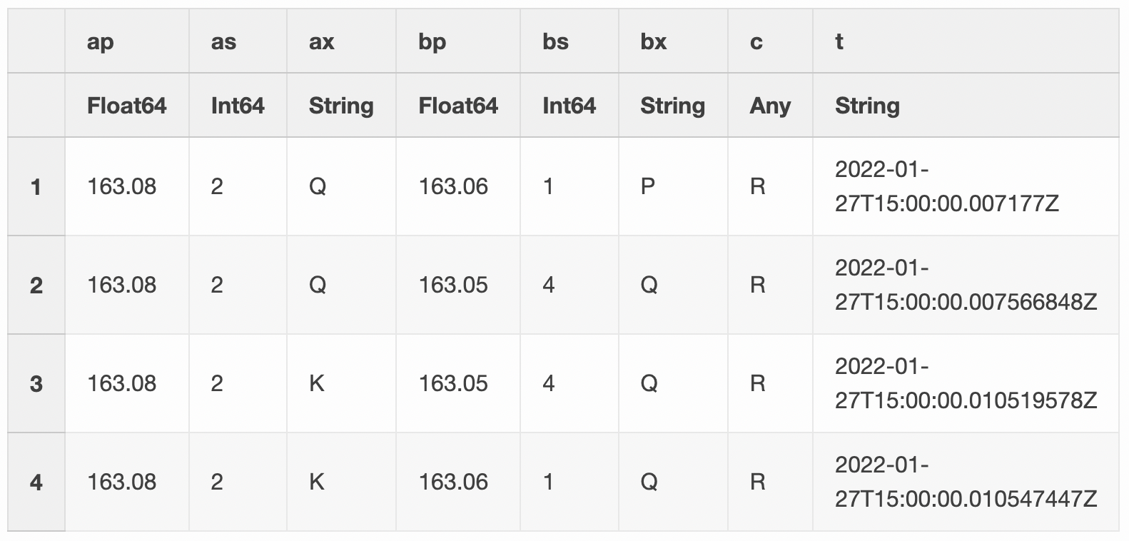
If we look at just one second’s worth of quotes, we get quite a bit of data.

aapl = AlpacaMarkets.get_stock_quotes("AAPL", 
  DateTime("2022-01-27T15:00:00"),
  DateTime("2022-01-27T15:00:01"))
first(aapl, 3)

3 rows × 10 columns (omitted printing of 2 columns)

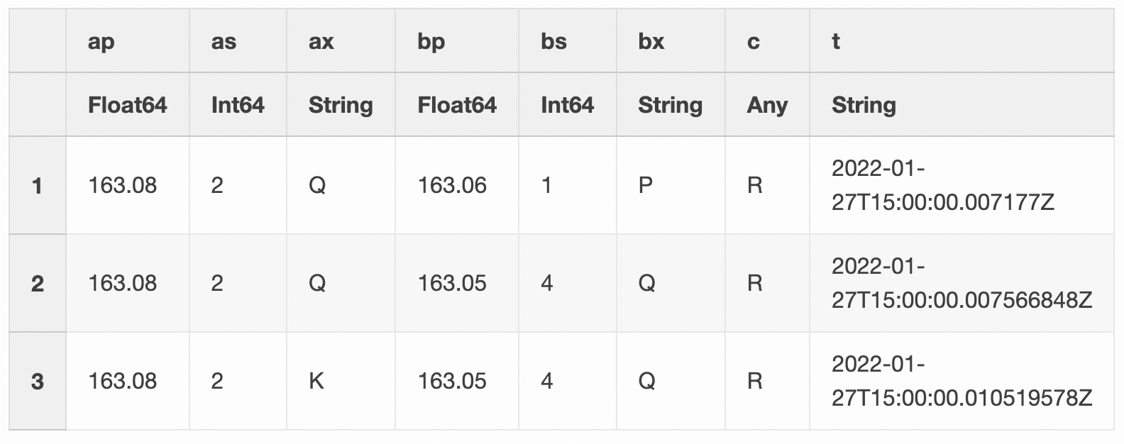
In the ax and bx columns (ask exchange and bid exchange), we can see what venue was offering that price at a given time. More on that later.

If we want to look at this data, we have to convert the timestamp into a Julia DateTime object. The values that come down the wire are a little funky, so I’ve written a help function in the AlpacaMarkets.jl module to help.

function convert_t_timestamp(x)
   ts =  first(x, 23)

    if endswith(ts, "Z")
        ts = chop(ts)
    end
    DateTime(ts)
end

function convert_t_time(x)
   ts = split(x, "T")[2]
   ts = first(ts, 12)
    if endswith(ts, "Z")
        ts = chop(ts)
    end
    Time(ts)
end

However, Julia’s default DateTime type only allows up millisecond precision. When we look at our data we have up to nanoseconds, so need to use the TimeDate.jl package to account for these extra digits.

aapl = @transform(aapl, :TimeStamp = convert_t_timestamp.(:t),
                        :TimeStamp_nano = TimeDate.(string.(chop.(:t))));

We now plot the bid and ask price.

ticks = minimum(aapl.TimeStamp):Millisecond(250):maximum(aapl.TimeStamp)
tick_labels = Dates.format.(ticks, "HH:MM:SS.sss")

plot(aapl.TimeStamp, aapl.ap, label = "Ask Price", seriestype=:steppre, xticks = (ticks, tick_labels))
plot!(aapl.TimeStamp, aapl.bp, label = "Bid Price", seriestype=:steppre)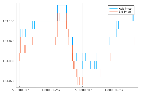

There we go - the movement of the best bid and ask price over one second. Most data sources would condense this into a single open-high-low-close bar, whereas AlpacaMarkets.jl is giving us the raw data underneath that data. All for free!

This means that you can calculate things like:

Quote intensity - how often there is a new price in a set period,
Order flow imbalance - how the supply and demand changes in the order book,
Tick by tick models - predicting what the next tick will be, easier than predicting what the next price will be.

I’ve written about Order flow imbalance before in the crypto markets. It's about looking at frequent changes in the best ask/offer and the amount that corresponds to these prices. Each small change gives us an idea of the supply and demand and can reasonably predict future price movements.

Overall, getting the raw best bid/offers from Alpaca across all these stocks is a treasure trove of information, and with my package you can easily save a database worth of data for your project.

Stock Trade Data

Alpaca also give us access to what trades, so stock transactions, happened over some time. This records how much stock was traded at a given time and for what price.

Again, we'll look at the same one-second period.

aaplTrades  = AlpacaMarkets.get_stock_trades("AAPL", DateTime("2022-01-27T15:00:00"), DateTime("2022-01-27T15:00:01"))
first(aaplTrades, 5)

5 rows × 8 columns

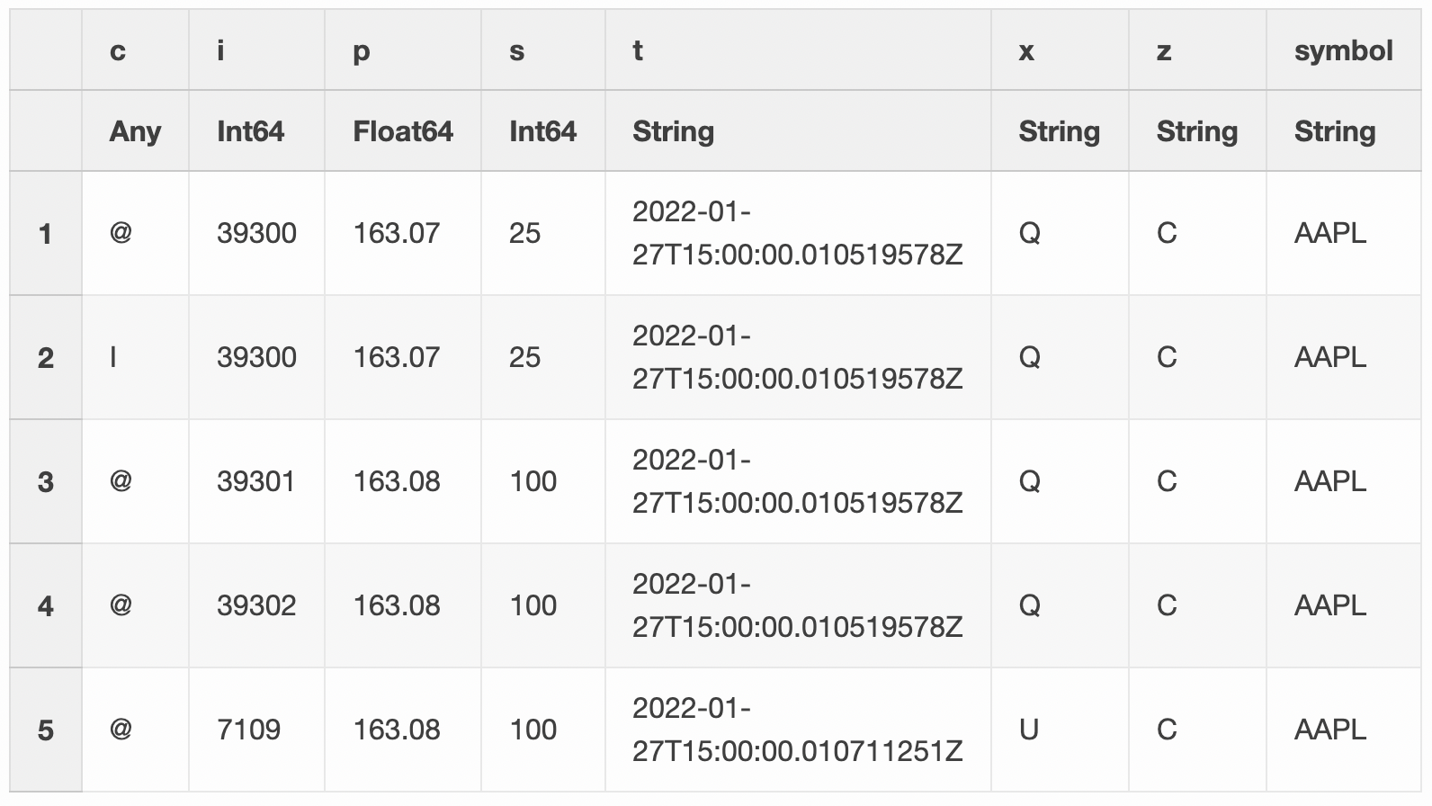
We can see a new column, c, which has different symbols for each row. This is the condition code and describes the type of trade. For the first two trades we see:

@ : is a regular trade
I: is an odd lot trade

The x column dictates where the trade happened, so the venue that executed the trade. The z column tells us what tape the trade was recorded on. There are three possible tapes, A, B, and C.

Again, we convert the timestamp and plot it against the prices. We also want just the unique trade ids (i) to make sure each trade is represented once.

aaplTrades = unique(aaplTrades, :i)
aaplTrades = @transform(aaplTrades, :TimeStamp = convert_t_timestamp.(:t),
                                    :TimeStamp_nano = TimeDate.(string.(chop.(:t))));

plot(aapl.TimeStamp, aapl.ap, label = "Ask Price", seriestype=:steppre, xticks = (ticks, tick_labels))
plot!(aapl.TimeStamp, aapl.bp, label = "Bid Price", seriestype=:steppre)
plot!(aaplTrades.TimeStamp, aaplTrades.p, label="Trades", seriestype=:scatter)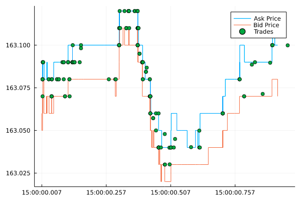

The trades line up nicely with the prices at the same time and we can see the series of trades that drove the price higher between 500 and 750 milliseconds past 15:00.

We’ve now got quite a complete picture of what happened in the second between 15:00:00 and 15:00:01.

344 price updates
384 trades

It’s now up to you to use that data how you see fit. Here I’ll demonstrate a few ideas.

Equity Venue Analysis

There are so many stock trading venues in the U.S., but what ones are good? If you’ve read Flash Boys, you might think they are all bad except for IEX. If you’ve read The Lean Startup you might think that the Long Term Stock Exchange is a good idea. But marketing and popularity aside, this is a key question for people who are fine-tuning their execution to ensure the best possible price.

Generally, we want to consider two things:

How long did they have the best price?
How much volume did they have at this best price?

So, using our quote data we can try and calculate some statistics.

Let’s pull some Apple quotes over one hour now.

aaplVenue = AlpacaMarkets.get_stock_quotes("AAPL", DateTime("2022-01-27T15:00:00"), DateTime("2022-01-27T16:00:00"))
first(aaplVenue, 4)

4 rows × 10 columns (omitted printing of 2 columns)

Using the TimeDate package, we can create an object with the correct resolution up to the nanosecond as reported by Alpaca Markets. We then calculate how long that price was the best bid or offer using diff.

function get_ns(x)
    getfield(x, :value)
end
    
aaplVenue = @transform(aaplVenue, :TimeStamp = convert_t_timestamp.(:t),
                                  :TimeStamp_nano = TimeDate.(string.(chop.(:t))));
aaplVenue = @transform(aaplVenue, :TimeDelta = [diff(:TimeStamp_nano); NaN])
aaplVenue = aaplVenue[1:(end-1), :]
aaplVenue = @transform(aaplVenue, :ns = get_ns.(:TimeDelta));

Now for each venue, plus bid and ask price, we group by the exchange and calculate the following:

How many times it was the best bid and best offer
The average number of shares available at this price
How long was the quote the best bid or offer.

This gives us three different values to assess the ‘quality’ of each venue.

gdata_bids = groupby(aaplVenue, :bx)
gdata_asks = groupby(aaplVenue, :ax)
venue_bids = @combine(gdata_bids, :n_best_bid = length(:c), 
                                  :avg_size_bid = mean(:as),
                                  :avg_time_best_bid = mean(:ns) * 1e-9)
venue_asks = @combine(gdata_asks, :n_best_ask = length(:c), 
                                  :avg_size_ask = mean(:as),
                                  :avg_time_best_ask = mean(:ns) * 1e-9)
rename!(venue_asks, ["venue", "n_best_ask", "avg_size_ask", "avg_time_best_ask"])
rename!(venue_bids, ["venue", "n_best_bid", "avg_size_bid", "avg_time_best_bid"])

venue = leftjoin(venue_bids, venue_asks, on = "venue")
venue = leftjoin(venue, rename!(AlpacaMarkets.STOCK_EXCHANGES, ["Name", "venue"]), on = "venue")

first(venue[!,["Name", "n_best_ask", "avg_size_ask", "avg_time_best_ask"]], 4)

4 rows × 4 columns

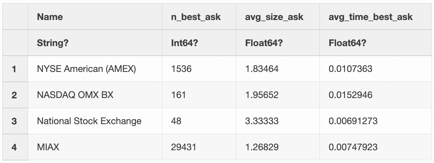
Plus all the values for the bid side too.

Now let’s visualize it with a quadrant plot.

plot(log.(venue.n_best_bid), venue.avg_size_bid, seriestype = :scatter, 
    label = :none, group = venue.venue, 
    series_annotations = text.(venue.Name, :bottom, pointsize=8),
    xlabel = "log (Number of Times Best Bid)",
    ylabel = "Average Bid Size")
hline!([mean(venue.avg_size_bid)], label=:none, color=:black)
vline!([mean(log.(venue.n_best_bid))], label=:none, color=:black)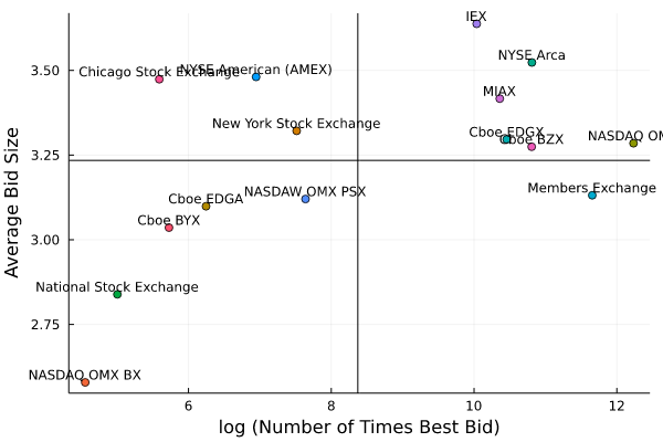

plot(log.(venue.n_best_ask), venue.avg_time_best_ask, seriestype = :scatter, 
    label = :none, group = venue.venue, 
    series_annotations = text.(venue.Name, :bottom, pointsize=8),
    xlabel = "log (Number of Times Best Ask)",
    ylabel = "Average Time Best Ask (seconds)")
hline!([mean(venue.avg_time_best_ask)], label=:none, color=:black)
vline!([mean(log.(venue.n_best_ask))], label=:none, color=:black)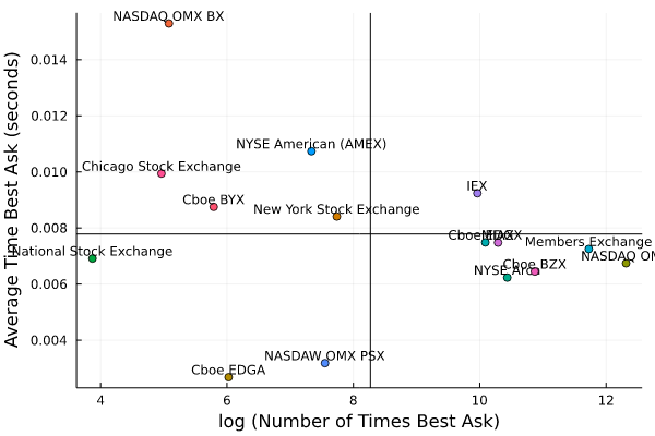

There are two clusters of exchanges and those to the right look like the best. They are top of book the most and also quote the largest size. To give an idea of size IEX quotes about 0.5 more shares than the Members Exchange. For Apple, with a share price of around $175, you can trade $87.5 more notional with IEX (on average) than the Members Exchange, so if you have a large order, it might mean going to the market fewer times and therefore paying fewer transaction costs.

OK, so that’s something interesting with the quotes. What about the trades?

The Lee-Ready Algorithm

When Alpaca sends us the trades, there is no indication if the trade was a buy or a sell. This can make analysis slightly harder, as we first have to try and guess the sign of the trade. If we look at the plot of the trades again, we can see that the trades happen predictably.

Most of the trades happen at the higher ask price, so they are probably buying, and likewise, some trades fall on the bid price line. These are probably sales.

Now, guessing what sign the trades has plenty of academic research behind it. One of the typical methods is the Lee-Ready algorithm which looks at where the trade is compared to the quoted mid-price at the time of the trade. If the trade is above the mid-price then it is likely that the trade was a buy and vice versa, if it was below it was likely a sell.

To evaluate this algorithm, we have to join the trades with the closest prices. Normally this would just be an ASOF join, but we have to hack our way around this in Julia.

tradeTimes = aaplTrades.TimeStamp_nano
quoteTimes = aapl.TimeStamp_nano

quoteInds = searchsortedlast.([quoteTimes], tradeTimes)

aaplTrades[!, "ap"] = aapl.ap[quoteInds]
aaplTrades[!, "bp"] = aapl.bp[quoteInds]

aaplTrades = @transform(aaplTrades, :Mid = (:ap .+ :bp) ./ 2)

aaplTrades[1:4, ["t", "TimeStamp_nano", "p", "ap", "bp", "Mid"]]

4 rows × 6 columns (omitted printing of 2 columns)

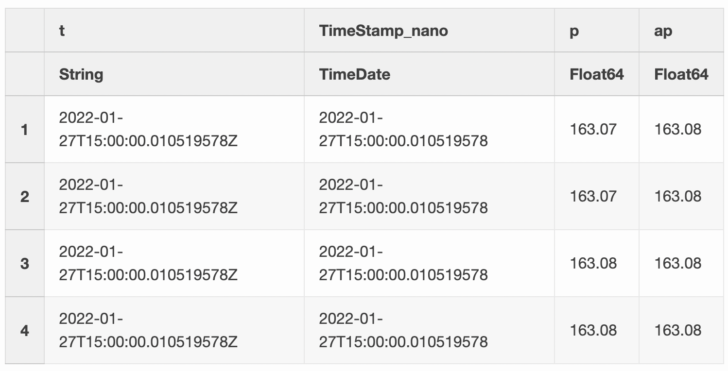
With the prices added, we check the sign of the difference between the traded price and the mid-price to classify it as a buy or sell.

function classify_trade(x)
    if x == 0
        return "Unknown"
    elseif x == 1
        return "Buy"
    else
        return "Sell"
    end
end


aaplTrades = @transform(aaplTrades, :Sign = sign.(:p .- :Mid))
aaplTrades = @transform(aaplTrades, :Side = classify_trade.(:Sign))


plot(aapl.TimeStamp, aapl.ap, label = "Ask Price", seriestype=:steppre, xticks = (ticks, tick_labels))
plot!(aapl.TimeStamp, aapl.bp, label = "Bid Price", seriestype=:steppre)
plot!(aaplTrades.TimeStamp, aaplTrades.p, seriestype=:scatter, groups=aaplTrades.Side)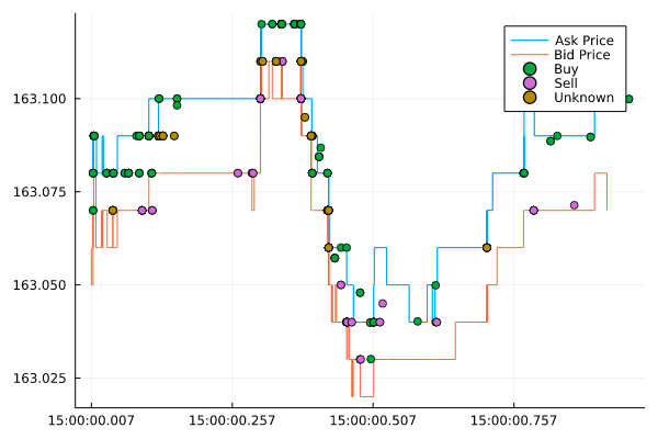

It’s not a 100% foolproof method, as we can see that it hasn’t managed to classify all the trades; some are unknown.

All investments involve risk and the past performance of a security, or financial product does not guarantee future results or returns.There is no guarantee that any investment strategy will be successful in achieving its investment objectives. Diversification does not ensure a profit or protection against a loss. There is always the potential of losing money when you invest in securities, or other financial products. Investors should consider their investment objectives and risks carefully before investing.

Alpaca does not prepare, edit, or endorse Third Party Content. Alpaca does not guarantee the accuracy, timeliness, completeness or usefulness of Third Party Content, and is not responsible or liable for any content, advertising, products, or other materials on or available from third party sites

Cryptocurrency is highly speculative in nature, involves a high degree of risks, such as volatile market price swings, market manipulation, flash crashes, and cybersecurity risks. Cryptocurrency is not regulated or is lightly regulated in most countries. Cryptocurrency trading can lead to large, immediate and permanent loss of financial value. You should have appropriate knowledge and experience before engaging in cryptocurrency trading. For additional information, please click here.

Community Examples