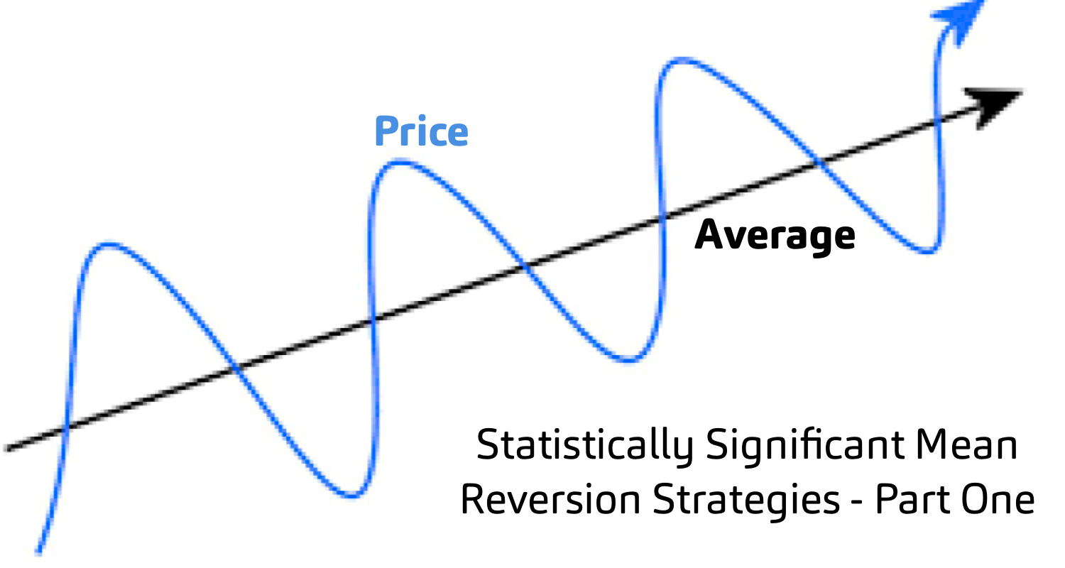
Statistically Significant Mean Reversion Strategies - Part One

21 Dec 2020

Statistical Arbitrage, often abbreviated as StatArb, is a class of mean-reversion trading strategies that involve data mining and statistical methods.

Hi, My name is Leo Smigel, and I'm an algorithmic trader. If you're new here, welcome. In this two-part series, I will show you how to create a statistically significant mean reversion strategy.

As always, all of the code examples will be in the Analyzing Alpha Github Repo, listed here:

Before we create a mean reversion strategy, we have to determine if a price series is stationary.

Stationarity

Understanding stationarity is essential as it's foundational to mean reversion trading.

A price series is stationary if it is mean-reverting, and the standard deviation stays relatively stable. This is critical to us as algorithmic traders. A stationary series current price can provide information into the likely direction of its future price.

Most instrument's prices are NOT stationary.

So how do we test if a time series is stationary?

The Augmented Dicky-Fuller test comes to the rescue.

Augmented Dicky-Fuller (ADF) Test

The ADF tests if a price series is NOT stationary (null hypothesis). We can use statsmodels using the adfuller function to either accept or reject this hypothesis. The best way to understand the ADF is to see it in action.

Let's grab our price data from alpaca using the Python SDK and determine if Google's price is stationary.

import alpaca_trade_api as tradeapi
api = tradeapi.REST(key_id="YOUR_API_KEY", secret_key="YOUR_SECRET_KEY")
barset = api.get_barset('GOOG', 'day', limit=252)

# Augmented Dicky-Fuller Test
from statsmodels.tsa.stattools import adfuller
r = adfuller(barset.df[('GOOG', 'close')].values)
print(f'ADF Statistic: {r[0]:.2f}') 
for k,v in r[4].items():   
	print (f'{k}: {v:.2f}')

ADF Statistic: -1.01
1%: -3.46
5%: -2.87
10%: -2.57

Notice that we can't reject the null hypothesis, that being the price series is not stationary, even at the 10% confidence level -- in other words, Google's price series is not mean-reverting.

So how do we find a mean-reverting series? Generally, we don't; however, we can create a cointegrated series. We can combine two or more non-stationary series into one potentially stationary 'spread' series.

Let's give this a shot with Home Depot and Lowes. We'll use code similar to the above to grab the price data.

hd = api.get_barset('HD', 'day', limit=252)
low = api.get_barset('LOW', 'day', limit=252)

Let's plot the prices to get an intuitive understanding of how these prices move together.

import matplotlib.pyplot as plt
plt.plot(hd.df[('HD','close')], c='red', label='HD')
plt.plot(low.df[('LOW','close')], c='blue', label='LOW')
plt.legend()
plt.show()

The prices are correlated but are they cointegrated?

The Cointegrated Augmented Dickey-Fuller (CADF) Test

We can use the Cointegrated Augmented Dickey-Fuller test. Here are the steps:

Determine the ratio to combine the two series. This ratio is called the hedge ratio.
Combine the two series using the hedge ratio. For example, buy one share of Google and sell two shares of Facebook.
Run an ADF test to determine stationarity.

The Hedge Ratio

We can calculate the hedge ratio using linear regression. Let's take the first 126 days of Home Depot and Lowe's price data. We'll use statsmodels once again. When determining the spread and stationarity, we'll avoid using data we used in our model to prevent look-ahead bias.

# let's align the indicies
i = hd.df.index.join(low.df.index, how='inner')
hddf = hd.df[('HD','close')].loc[i]
lowdf = low.df[('LOW','close')].loc[i]

# calculate the hedge ratio
import statsmodels.api as sm
model = sm.OLS(hddf[:126], lowdf[:126])
model = model.fit()
hedge_ratio = model.params[0]
print(f'Hedge Ratio: {hedge_ratio:.2f}')

# plot scatter
plt.scatter(hd.df[('HD','close')][126:], low.df[('LOW','close')][126:])
plt.xlabel('Home Depot')
plt.ylabel('Lowes')
plt.show()

# determine the spread
spread = hddf[:126] - hedge_ratio * lowdf[:126]

Let’s plot the spread to see if it looks mean-reverting.

The above doesn’t look promising. Let’s back-up this assertion with an ADF test.

# determine stationarity
r = adfuller(spread)
print(f'ADF Statistic: {r[0]:.2f}')
for k,v in r[4].items():
	print (f'{k}: {v:.2f}')

ADF Statistic: -1.64
1%: -3.48
5%: -2.88
10%: -2.58

Unfortunately, the combination is not stationary, which means we shouldn't use it for a mean reversion strategy -- at least not at the moment. Many price series will fall in and out of cointegration.

In the next post, we will continue learning how to create statistically significant mean reversion strategies. Until then, try to discover a stationary spread and check out Analyzing Alpha.

Again all of the code from this tutorial series can be found on the following GitHub repository:

Technology and services are offered by AlpacaDB, Inc. Brokerage services are provided by Alpaca Securities LLC (alpaca.markets), member FINRA/SIPC. Alpaca Securities LLC is a wholly-owned subsidiary of AlpacaDB, Inc.

You can find us @AlpacaHQ, if you use twitter.