Statistically Significant Mean Reversion Strategies - Part Two

18 Jan 2021

Statistically Significant Mean Reversion Strategies

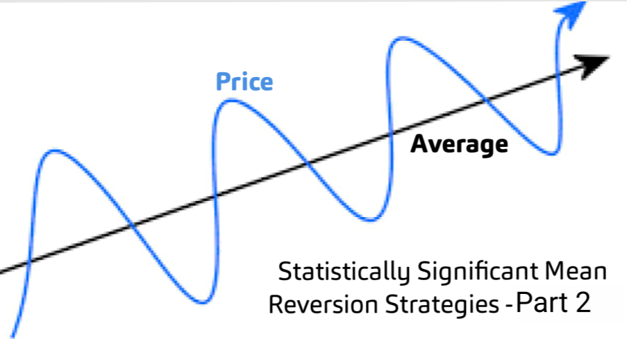
Welcome back to part two of this series on using statistical arbitrage to develop mean reversion trading strategies, also known as StatArb.

My name is Leo Smigel, and I enjoy the puzzle of creating algorithmic trading strategies, which I write about at analyzingalpha.com.

Previously, we discussed what cointegration is and how it can help us potentially profit in the market. Part 1 of the series can be found below:

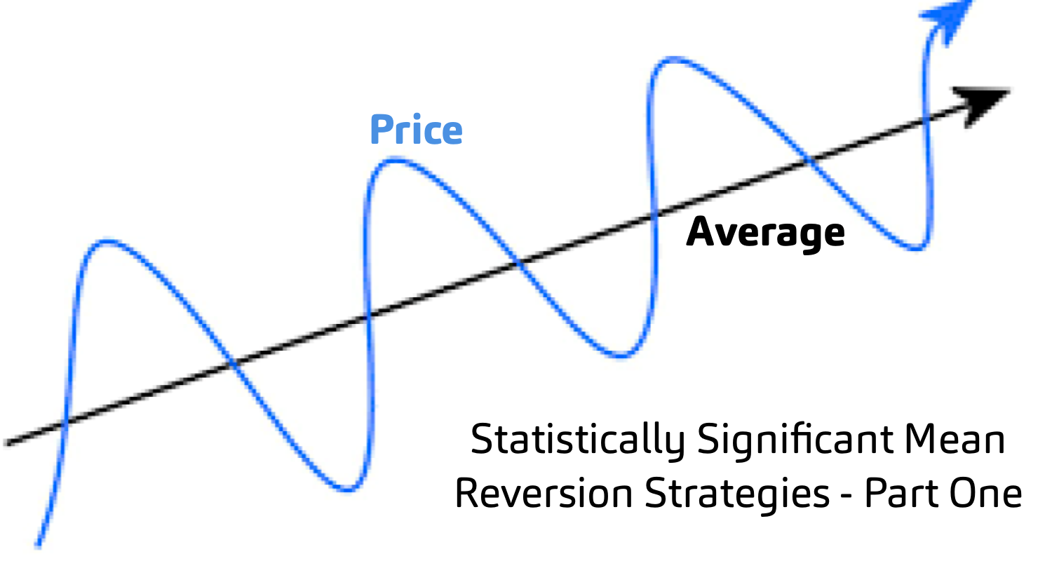
This post will learn how to create a statistically significant mean reversion strategy that uses more than two assets.

Start With Why

When developing algorithmic trading strategies, It's important to understand why the strategy should work and not that it "just does" to reduce overfitting and increase conviction.

Let's discuss an example put forth by Ernie Chan in his book Algorithmic Trading: Winning Strategies and Their Rationale.

The price and profitability of gold miners are highly dependent on the price of gold. If the price of gold goes up, gold miners are more profitable. When the price of gold goes down, they make less money. This relationship is easy to understand and makes intuitive sense -- and it's also backed up by the data.

Between May 23, 2006, and July 14, 2008, gold prices (GLD) and gold miners (GDX) cointegrate with 99% probability!.. until they didn't.

Gold and GDX lost their cointegration. But why?

Black Gold

The price of black gold, also known as oil, skyrocketed around that period. And since extracting gold uses a lot of oil, it hurt the gold miner's profitability.

Makes sense, right?

The good news is that we can adjust our strategy to add USO to our pair, which is also known as a triplet.

Trading Triplets

The Cointegrated Augmented Dicky-Fuller test won't work for us. We need a test that can use more than two assets -- enter the Johansen test.

The Johansen test allows us to test for cointegration for multiple time series. And while we won't get into how this vector error correction model works, I suggest you get a deep understanding if you start using Johansen tests to develop live trading strategies.

Let's start with grabbing our data from Alpaca and aligning the dates.

# Get data from alpaca and align dates
gld = api.get_barset('GLD', 'day', limit=252)
gdx = api.get_barset('GDX', 'day', limit=252)
uso = api.get_barset('USO', 'day', limit=252)

glddf = gld.df[('GLD', 'close')].rename("GLD")
gdxdf = gdx.df[('GDX', 'close')].rename("GDX")
usodf = uso.df[('USO', 'close')].rename("USO")

glddf = glddf.to_frame()
df = glddf.join([gdxdf, usodf], how='inner')

Get data from alpaca and align dates

Let's visualize the data to see if everything looks correct.

Hmmm, it looks like there was a significant price change in oil in late April. More on this later.

# Johansen Test
from statsmodels.tsa.vector_ar.vecm import coint_johansen
r = coint_johansen(df, 0, 1)

# Print trace statistics and eigen statistics
print(f"\t\tStat \t90%\t 95%\t 99%")
print (f"R <= Zero\t{round(r.lr1[0], 3)}\t{round(r.cvt[0, 0], 3)}\t {round(r.cvt[0, 1],3)}\t {round(r.cvt[0, 2],3)}")

Johansen Test

We get the following output:

    	Stat     90%     95%     99%
R <= Zero    20.089    27.067     29.796     35.463

Trace Statistics

We're looking for our trace statistic currently 20.089, to be above the critical values at the 90%, 95%, and 99% threshold. Unfortunately, they're not. So while this triplet strategy used to work, it doesn't work now, or does it?

The Challenges of Live Data

The problem with live data is that it isn’t adjusted. When I look at the data adjusted for splits, dividends, and corporate actions, it looks vastly different.

# Analyze USO split
print(usodf['2020-04-25':'2020-04-30'])

Print Data

time
2020-04-27 00:00:00-04:00 	2.180
2020-04-28 00:00:00-04:00 	2.135
2020-04-29 00:00:00-04:00	17.780
2020-04-30 00:00:00-04:00	19.220
Name: USO, dtype: float64

USO Data

Look at the jump on the 28th - 29th, it appears as though there was an 8-for-1 reverse split on April 29th.

Stat              90%       95%       99%
R <= 0 30.25   27.067    29.796    35.463

Trace Statistics

With the adjusted data, it appears as though we can reject that the assets are not cointegrated with over 95% certainty!

In other words, you have to develop and backtest on adjusted data, and trade on live data. So if we were trading this strategy, what would that look like?

# Store result, eigenvector, and take strongest cointegrated spread
r = coint_johansen(df[:90], 0, 1) # Only use first 90 days
ev = result.evec
ev = result.evec.T[0]
ev = ev/ev[0]

Store result, eigenvector, and take strongest cointegrated spread

# Print the mean reverting spread
print(f"Spread: {ev[0]} GLD + {ev[1]} GDX + {ev[2]} USO")

Print Mean Reverting Spread

Spread: 1.0 GLD + -1.1422182979992972 GDX + -0.14004473766799466 USO

Spread

Next Steps

If you've made it this far, you've probably realized determining if assets are cointegrated using Python is the easy part -- the hard part is finding cointegrations and wrangling the data.

To trade this strategy, you would trade the spread when it moves X standard deviations away from the mean. The strategy can easily be tested in Pandas, Backtrader or QuantConnect.

I will leave this up to you to develop a trading strategy around this cointegrating triplet. I suggest using Pandas to prototype, and then use Backtrader or QuantConnect to further analyze and live trade.

Also, if you enjoy algorithmic trading, please check out Analyzing Alpha for more information on mean reversion strategies -- there’s a lot more to them.

And as always, all of the code is hosted on GitHub.

Technology and services are offered by AlpacaDB, Inc. Brokerage services are provided by Alpaca Securities LLC (alpaca.markets), member FINRA/SIPC. Alpaca Securities LLC is a wholly-owned subsidiary of AlpacaDB, Inc.

You can find us @AlpacaHQ, if you use twitter.