Crypto

How To Trade Crypto Using Machine Learning

19 Sep 2022

What is Machine Learning?

Machine learning is a branch of Artificial Intelligence (AI) and computer science that focuses on the use of data and algorithms to imitate the way humans learn, gradually improving its accuracy.1 Machine learning empowers traders to accelerate and automate one of the most complex, time-consuming, and challenging aspects of algorithmic trading, providing a competitive advantage beyond rules-based trading. 2

There are several kinds of machine learning algorithms that exist today for a range of use cases. We will be focusing on Long Short-Term Memory (LSTM).

What is LSTM?

LSTM is a special kind of recurrent neural network capable of handling long-term dependencies. These networks are capable of learning order dependence in sequence prediction problems.3 Financial time series prediction is one such problem where we can use LSTM to predict future prices of an asset. If you're interested in understanding how the network works, this article is a great resource.

What are we building?

We're building a trading bot that uses a LSTM model to predict the closing price of ETH/USD on Alpaca. We'll use market data from Alpaca to train our model and use the predicted closing price from the trained model to make necessary trading decisions. To start, we can consider two scenarios:

If we do not have a position and the current price of the asset is less than the predicted price of the asset at some time in the future. In this scenario, we place a BUY market order for a fixed quantity of the asset.
If we do have a position and the current price of the asset is more than the predicted price of the asset at some time in the future. In this scenario we place a SELL market order for a fixed quantity of the asset.

Let’s Build

Before getting started, you need to create an Alpaca account to use paper trading as well as fetch market data for ETH/USD. You can get one by signing up here. Code for this trading bot can be found here. Now, let’s get started!

from alpaca.data.historical import CryptoHistoricalDataClient
from alpaca.data.requests import CryptoBarsRequest
from alpaca.data.timeframe import TimeFrame
from alpaca.trading.client import TradingClient
from alpaca.trading.requests import MarketOrderRequest
from alpaca.trading.enums import OrderSide, TimeInForce
from datetime import datetime
from dateutil.relativedelta import relativedelta
from tensorflow.keras.models import Sequential
from tensorflow.keras.layers import Activation, Dense, Dropout, LSTM
from sklearn.preprocessing import MinMaxScaler
import matplotlib.pyplot as plt
import numpy as np
import pandas as pd
from sklearn.metrics import mean_absolute_error
import json
import logging
import config
import asyncio
 
 
# ENABLE LOGGING - options, DEBUG,INFO, WARNING?
logging.basicConfig(level=logging.INFO,
                   format='%(asctime)s - %(name)s - %(levelname)s - %(message)s')
logger = logging.getLogger(__name__)
 
 
# Alpaca Trading Client
trading_client = TradingClient(
   config.APCA_API_KEY_ID, config.APCA_API_SECRET_KEY, paper=True)

Start by importing the necessary libraries including Alpaca-py, Tensorflow and Sci-kit Learn (Sklearn). Alpaca-py is the latest official python SDK from Alpaca. It gives us the necessary market data and trading endpoints. We enable logging to monitor the latest prices and bot status.

Also, we define our trading client using Alpaca-py. It is currently set to using a paper environment. This can be easily set to use a live trading environment by setting the paper parameter as False.

# Trading variables
trading_pair = 'ETH/USD'
qty_to_trade = 5
# Wait time between each bar request and model training
waitTime = 3600
data = 0
current_position, current_price = 0, 0
predicted_price = 0

Next, define some trading variables that we will use to trade ETH/USD. This includes our trading pair ETH/USD, the quantity of ETH we would like to buy for each trade, our current position, current price of the asset and the predicted price of the asset.

async def main():
   '''
   Function to get latest asset data and check possible trade conditions
   '''
 
   # closes all position AND also cancels all open orders
   # trading_client.close_all_positions(cancel_orders=True)
   # logger.info("Closed all positions")
 
   while True:
       logger.info('--------------------------------------------')
       pred = stockPred()
       global predicted_price
       predicted_price = pred.predictModel()
       logger.info("Predicted Price is {0}".format(predicted_price))
       l1 = loop.create_task(check_condition())
       await asyncio.wait([l1])
       await asyncio.sleep(waitTime)

Let’s talk about what our main function does. It runs a never ending loop that predicts the price of our asset ETH/USD at a later point in time and makes trading decisions based on the predicted price, current price of the asset and position of the asset in our account.

We start by creating an instance of class stockPred and call it pred. We then call the predictModel() method that returns the predicted price of ETH/USD at a later point in time.

Once we have the predicted price, we call the function check_condition() that computes if a trade should be made. After waiting for a waitTime amount of seconds this process repeats again. We have set the waitTime to 3600 seconds to wait for 1hr before we check for a trade again. This can be changed based on the timeframe of data you are looking at. Since we are considering an hourly timeframe and predicting the closing price of ETH/USD one hour into the future, it is reasonable to keep it at 3600 seconds.

Next, let’s explore the class stockPred. While building this prediction class, I took inspiration from work found here. 4 It was of great help in creating this model and defining the necessary parameters. It has a few functions so we will look at them in snippets.

class stockPred:
   def __init__(self,
             past_days: int = 50,
             trading_pair: str = 'ETHUSD',
             exchange: str = 'FTXU',
             feature: str = 'close',
             look_back: int = 100,
             neurons: int = 50,
             activ_func: str = 'linear',
             dropout: float = 0.2,
             loss: str = 'mse',
             optimizer: str = 'adam',
             epochs: int = 20,
             batch_size: int = 32,
             output_size: int = 1
             ):
    self.exchange = exchange
    self.feature = feature
    self.look_back = look_back
    self.neurons = neurons
    self.activ_func = activ_func
    self.dropout = dropout
    self.loss = loss
    self.optimizer = optimizer
    self.epochs = epochs
    self.batch_size = batch_size
    self.output_size = output_size

The __init__() method initializes the variables needed to filter our market data and train the LSTM model. These include parameters like lookback period (period to consider in the past to make a future prediction), number of neurons/nodes that will be part of each layer of our LSTM mode, loss function, activation function, number of epochs to train our model for, optimizer, batch size and the output size.

def getAllData(self):
    # Alpaca Market Data Client
    data_client = CryptoHistoricalDataClient()
 
    time_diff = datetime.now() - relativedelta(hours=1000)
    logger.info("Getting bar data for {0} starting from {1}".format(trading_pair, time_diff))
    # Defining Bar data request parameters
    request_params = CryptoBarsRequest(
        symbol_or_symbols=[trading_pair],
        timeframe=TimeFrame.Hour,
        start=time_diff)
 
    # Get the bar data from Alpaca
    df = data_client.get_crypto_bars(request_params).df
    global current_price
    current_price = df.iloc[-1]['close']
    return df
 
def getFeature(self, df):
    data = df.filter([self.feature])
    data = data.values
    return data

getAllData() method helps us get the raw market data that we need to train the model. First, it instantiates a data client using Alpaca-py. Then we create a CryptoBarRequest() and pass in the necessary parameters like symbol, timeframe of the data we would like and the start time of the data. Since we are trading ETH/USD, the symbol parameter is ETHUSD for the market data request. We are also requesting the data to be in hourly time frame and start 1000 hours before the current time. Keep in mind that the current time in your time zone might result in a different number of rows.

These parameters can be optimized further for better performance. Passing in the request we just created to the get_crypto_bars() method returns the needed bar data. Now that we have the necessary bar data, we set the current price of the asset to be the last closing price in the bar data and finally return the bar data of the asset.
getFeature() method extracts the price column we are looking to predict. Since we are looking to predict the closing price of Ethereum, we filter only the ‘close’ column of the bar data and return it.

def scaleData(self, data):
    scaler = MinMaxScaler(feature_range=(-1, 1))
    scaled_data = scaler.fit_transform(data)
    return scaled_data, scaler
 
# train on all data for which labels are available (train + test from dev)
def getTrainData(self, scaled_data):
    x, y = [], []
    for price in range(self.look_back, len(scaled_data)):
        x.append(scaled_data[price - self.look_back:price, :])
        y.append(scaled_data[price, :])
 
    return np.array(x), np.array(y)

scaleData() helps us transform our bar data we just requested from Alpaca. Why is scaling important in machine learning? This is because the machine is just looking at numbers. It doesn’t understand the importance or relative distinction between high or low numbers. In this case, outliers might skew the interpretation of the data in a certain direction resulting in a biased output. To help scale the data, we use sklearn’s MinMaxScaler() method to scale our closing prices in the range (-1,1).

getTrainData() is one of the most important methods in the class. It creates the shape of our training data. If we are looking at market data 1000 hours in the past from our current time with each hour being its own row, then it will create a 3D array of size (900,100,1). This means it will create 900 samples with each sample being 100 hours to look in the back (look_back) and 1 forward looking result value.

def LSTM_model(self, input_data):
    model = Sequential()
    model.add(LSTM(self.neurons, input_shape=(
        input_data.shape[1], input_data.shape[2]), return_sequences=True))
    model.add(Dropout(self.dropout))
    model.add(LSTM(self.neurons, return_sequences=True))
    model.add(Dropout(self.dropout))
    model.add(LSTM(self.neurons))
    model.add(Dropout(self.dropout))
    model.add(Dense(units=self.output_size))
    model.add(Activation(self.activ_func))
    model.compile(loss=self.loss, optimizer=self.optimizer)
    return model

The code snippet above creates our LSTM model. It starts by instantiating a Sequential model and followed by adding LSTM layers on it. We need to specify the number of neurons in each LSTM layer. In this example, we are using 50 neurons for each LSTM layer. A LSTM layer is usually followed by a Dropout layer. The Dropout layer randomly sets input units to 0 with a frequency of rate at each step during training time, which helps prevent overfitting.5 In total 3 LSTM layers are added followed by a Dropout layer each. This is followed by adding a final Dense layer and then passing the result through an activation function. We are using a linear activation function here. Now that the model is created, we can configure the model with the loss function and optimizer we would like to use. We are using the Mean Squared Error loss function and Adam optimizer in our example.

def trainModel(self, x, y):
       x_train = x[: len(x) - 1]
       y_train = y[: len(x) - 1]
       model = self.LSTM_model(x_train)
       modelfit = model.fit(x_train, y_train, epochs=self.epochs,
                            batch_size=self.batch_size, verbose=1, shuffle=True)
       return model, modelfit

trainModel() uses the x and y arrays from getTrainData() method to feed the training data to our LSTM model we created in the previous snippet and then trains it. The necessary training data x_train and y_train are extracted from the arrays that are fed in. Calling model.fit() method trains our model on the training data we just prepared. Along with the training data, we pass it the number of epochs we need our model to train and the batch size of the data being fed. Epoch defines the number of times we go through training while batch size defines the number of samples processed before the model is updated. The size of a batch must be more than or equal to one and less than or equal to the number of samples in the training dataset.6

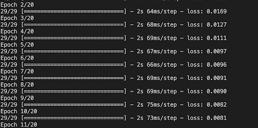
The image above shows what a model being trained might look like. Since we set the number of Epochs to 20, we can expect the model to go through our data 20 times.

def predictModel(self):
       logger.info("Getting Ethereum Bar Data")
       # get all data
       df = self.getAllData()
 
       logger.info("Getting Feature: {}".format(self.feature))
       # get feature (closing price)
       data = self.getFeature(df)
 
       logger.info("Scaling Data")
       # scale data and get scaler
       scaled_data, scaler = self.scaleData(data)
 
       logger.info("Getting Train Data")
       # get train data
       x_train, y_train = self.getTrainData(scaled_data)
 
       logger.info("Training Model")
       # Creates and returns a trained model
       model = self.trainModel(x_train, y_train)[0]
 
       logger.info("Extracting data to predict on")
       # Extract the Closing prices that need to be fed into predict the result
       x_pred = scaled_data[-self.look_back:]
       x_pred = np.reshape(x_pred, (1, x_pred.shape[0]))
 
       # Predict the result
       logger.info("Predicting Price")
       pred = model.predict(x_pred).squeeze()
       pred = np.array([float(pred)])
       pred = np.reshape(pred, (pred.shape[0], 1))
 
       # Inverse the scaling to get the actual price
       pred_true = scaler.inverse_transform(pred)
       return pred_true[0][0]

The code snippet above calls all the functions we defined above in the class. It starts by getting the necessary bar data for our asset, ETH/USD. This is followed by extracting the feature (closing price), scaling the data and then extracting the training data for our model. Once we have the training data ready, trainModel() is called. It creates and trains the model with the parameters we define along with feeding it the training data.

Now that we have our model trained, we also need to prepare the data that we need to predict on. For this we select the last 100 hours (look_back period) of data to look back at to predict 1 hour into the future. Remember, we only had 900 samples in our training data? The last 100 samples are to predict the next hour’s closing price.Once the data we need to predict on, is ready, we can execute the coolest part of the entire bot, predicting the closing price of Ethereum for the next hour. This is done by calling model.predict() method. The result from this operation is then reshaped. Remember that the data we have been feeding the model and its output are still scaled. This means they lie in the range (-1,1). Now that we have our result in this range, we can inverse transform it using the scaler object we used to scale our data in the first place. This returns our true predicted closing price for the next hour.

async def check_condition():
   '''
   Strategy:
   - If the predicted price an hour from now is above the current price and we do not have a position, buy
   - If the predicted price an hour from now is below the current price and we do have a position, sell
   '''
   global current_position, current_price, predicted_price
   current_position = get_positions()
   logger.info("Current Price is: {0}".format(current_price))
   logger.info("Current Position is: {0}".format(current_position))
   # If we do not have a position and current price is less than the predicted price place a market buy order
   if float(current_position) <= 0.01 and current_price < predicted_price:
       logger.info("Placing Buy Order")
       buy_order = await post_alpaca_order('buy')
       if buy_order:  
           logger.info("Buy Order Placed")
 
   # If we do have a position and current price is greater than the predicted price place a market sell order
   if float(current_position) >= 0.01 and current_price > predicted_price:
       logger.info("Placing Sell Order")
       sell_order = await post_alpaca_order('sell')
       if sell_order:
           logger.info("Sell Order Placed")

The code snippet above handles the trading logic for our bot. It takes into account the current price, predicted price of ETH/USD pair and also its position in our Alpaca account.

The logic states that if we do not have a position and the current price of Ethereum is less than its predicted price one hour from now, then we buy 5 ETH/USD. Since we are testing this on a paper trading account, we can trade any arbitrary amount greater than the minimum amount required to trade on Alpaca. The minimum amount of Ethereum we can trade on Alpaca is 0.01 ETH. Information about other cryptocurrencies and their minimum tradable quantity on Alpaca can be found here.

On the other hand, if we have an ETH/USD position and the predicted price of Ethereum is below its current price, we choose to sell.

More checks and balances can be added to optimize trading performance in the snippet above. For example, one might consider calculating fees involved in executing trades, loss cutting or even adding a minimum profit threshold. Some of these optimizations have been introduced in the Scalping article.

async def post_alpaca_order(side):
   '''
   Post an order to Alpaca
   '''
   try:
       if side == 'buy':
           market_order_data = MarketOrderRequest(
               symbol="ETHUSD",
               qty=qty_to_trade,
               side=OrderSide.BUY,
               time_in_force=TimeInForce.GTC
           )
           buy_order = trading_client.submit_order(
               order_data=market_order_data
           )
           return buy_order
       else:
           market_order_data = MarketOrderRequest(
               symbol="ETHUSD",
               qty=current_position,
               side=OrderSide.SELL,
               time_in_force=TimeInForce.GTC
           )
           sell_order = trading_client.submit_order(
               order_data=market_order_data
           )
           return sell_order
   except Exception as e:
       logger.exception(
           "There was an issue posting order to Alpaca: {0}".format(e))
       return False

Now, let's go through how the order execution works for this bot. Based on the side of the trade, we create a market order request using Alpaca-py's MarketOrderRequest() method. Here, we can specify the symbol of the asset, quantity of the asset we would like to trade, the side of the trade and time till when the order should stay in place (time_in_force). More information on the method and its arguments can be found here. The market order request we just created can then be submitted as an order using our trading client's submit_order() method. Once the orders are placed, we return the response object from Alpaca.

def get_positions():
   positions = trading_client.get_all_positions()
   global current_position
   for p in positions:
       if p.symbol == 'ETHUSD':
           current_position = p.qty
           return current_position
   return current_position

The snippet above is a helper function that returns the current position of ETH/USD pair in our account. It uses the get_all_positions() method from our trading client to retrieve the position and then assigns it to current_position.

loop = asyncio.get_event_loop()
loop.run_until_complete(main())
loop.close()

Finally, we use the asyncio module to run our main function in a loop.

Takeaway

Using neural networks to analyze market data and trading decisions can be a powerful and competitive tool for any trader. No model is absolutely perfect and should be tested in a paper environment before being deployed in a production environment with real money.

The model and data preparation we discussed in this article can be optimized further for better results. You can consider adding more layers or even experimenting with the model parameters. Working with different versions of the model can give a better understanding of what works on the asset you are trying to trade too.

If you are a M1 Mac user, you might need to set up Tensorflow this way. 7

Sources

Please note that this article is for informational purposes only. The example above is for illustrative purposes only. Actual crypto prices may vary depending on the market price at that particular time. Alpaca Crypto LLC does not recommend any specific cryptocurrencies.

Cryptocurrency is highly speculative in nature, involves a high degree of risks, such as volatile market price swings, market manipulation, flash crashes, and cybersecurity risks. Cryptocurrency is not regulated or is lightly regulated in most countries. Cryptocurrency trading can lead to large, immediate and permanent loss of financial value. You should have appropriate knowledge and experience before engaging in cryptocurrency trading. For additional information please click here.

Cryptocurrency services are made available by Alpaca Crypto LLC ("Alpaca Crypto"), a FinCEN registered money services business (NMLS # 2160858), and a wholly-owned subsidiary of AlpacaDB, Inc. Alpaca Crypto is not a member of SIPC or FINRA. Cryptocurrencies are not stocks and your cryptocurrency investments are not protected by either FDIC or SIPC. Please see the Disclosure Library for more information.

This is not an offer, solicitation of an offer, or advice to buy or sell cryptocurrencies, or open a cryptocurrency account in any jurisdiction where Alpaca Crypto is not registered or licensed, as applicable.

Crypto Trading API