Please note that this article is for educational and informational purposes only. All screenshots are for illustrative purposes only. The views and opinions expressed are those of the author and do not reflect or represent the views and opinions of Alpaca. Alpaca does not recommend any specific securities or investment strategies. Investing and investment strategies involve risk, including loss of value and the loss of principal. Past performance does not guarantee future returns or results. Please consider your objectives before investing.
This article first appeared on Medium, written by Victor S.
There are so many articles on predicting stock prices, but this article provides two things to the reader, that no other article talks about:
- The use of confidence intervals in stock trading to determine stop-loss and take-profit
- The use of Alpaca in stock trading to track profits and test trading strategies
Both of which provide important tools to the next generation of machine learning trading algorithms.
Concept:
The program will consist of three main parts:
- The Data Setup
The data will be accessed via the yfinance library, in daily intervals, The data will include the opening,high,low and closing price of the asset. The data will be normalized and then reshaped to fit the neural network
- The Neural Network
The neural network will be a convolutional LSTM network that can extract the feature and also access temporal features of the dataset. This network fits the data because some of the complex patterns are not only convolutional, they are also time based.
- Creating Orders
The Neural Network will predict the daily opening and closing prices. If the opening prices is larger than the closing price, the network will short sell the stock. If the closing price is larger than the opening price, the network will buy the stock.
After training the network, I will compute the loss of the network and use this value as a a confidence interval, to determine the stop loss and take profit values. I will use requests to access the Alpaca API to make orders.
With the key concept in place, let’s move to the code.
The Code
Step 1 | Prerequisites:
from numpy import array
from numpy import hstack
from keras.models import Sequential
from keras.layers import LSTM
from keras.layers import Dense
from keras import callbacks
from sklearn.model_selection import train_test_split
from keras.layers import Flatten
from keras.layers import TimeDistributed
from keras.layers.convolutional import Conv1D
from keras.layers.convolutional import MaxPooling1D
from IPython.display import clear_output
import datetime
import statistics
import time
import os
import json
import yfinance as yf
from keras.models import model_from_json
import requests
from keras.models import load_model
from matplotlib import pyplot as plt
There are quite a lot of prerequisties of the program.They are spread out as so, to prevent importing the whole library and taking up space. Please note that importing clear_output from IPython.display is only for Jupyter notebooks. If you are using scripts it is not necessary to import this.
Step 2 | Access Data:
def data_setup(symbol,data_len,seq_len):
    end = datetime.datetime.today().strftime('%Y-%m-%d')
    start = datetime.datetime.strptime(end, '%Y-%m-%d') - datetime.timedelta(days=(data_len/0.463))
    orig_dataset = yf.download(symbol,start,end)
    close = orig_dataset['Close'].values
    open_ = orig_dataset['Open'].values
    high = orig_dataset['High'].values
    low = orig_dataset['Low'].values
    dataset,minmax = normalize_data(orig_dataset)
    cols = dataset.columns.tolist()

    data_seq = list()
    for i in range(len(cols)):
        if cols[i] < 4:
            data_seq.append(dataset[cols[i]].values)
            data_seq[i] = data_seq[i].reshape((len(data_seq[i]), 1))
    data = hstack(data_seq)
    n_steps = seq_len
    X, y = split_sequences(data, n_steps)
    n_features = X.shape[2]
    n_seq = len(X)
    n_steps = seq_len
    print(X.shape)
    X = X.reshape((n_seq,1, n_steps, n_features))
    true_y = []
    for i in range(len(y)):
        true_y.append([y[i][0],y[i][1]])
    return X,array(true_y),n_features,minmax,n_steps,close,open_,high,low
This function takes data from yfinance and splits it into its respective sections. It also reshapes data into the form:
(n_seq,1, n_steps, n_features)A four-dimensional array to fit the Convolutional LSTM network.
Step 3 | Prepare Data:
Accessing the data is only half of the challenge. The rest is putting the data into the correct format, and splitting the data into training and testing datasets.
def split_sequences(sequences, n_steps):
        X, y = list(), list()
        for i in range(len(sequences)):
            end_ix = i + n_steps
            if end_ix > len(sequences)-1:
                break
            seq_x, seq_y = sequences[i:end_ix, :], sequences[end_ix, :]
            X.append(seq_x)
            y.append(seq_y)
        return array(X), array(y)
This function splits the sequence into time series data, by splitting the sequence into chunks of size n_steps.
def normalize_data(dataset):
        cols = dataset.columns.tolist()
        col_name = [0]*len(cols)
        for i in range(len(cols)):
            col_name[i] = i
        dataset.columns = col_name
        dtypes = dataset.dtypes.tolist()
#         orig_answers = dataset[attr_row_predict].values
        minmax = list()
        for column in dataset:
            dataset = dataset.astype({column: 'float32'})
        for i in range(len(cols)):
            col_values = dataset[col_name[i]]
            value_min = min(col_values)
            value_max = max(col_values)
            minmax.append([value_min, value_max])
        for column in dataset:
            values = dataset[column].values
            for i in range(len(values)):
                values[i] = (values[i] - minmax[column][0]) / (minmax[column][1] - minmax[column][0])
            dataset[column] = values
        dataset[column] = values
        return dataset,minmax
This function changes all data into a value between 0 and 1. This is as many stocks have skyrocketed or nosedived. Without normalizing, the neural network would learn from datapoints with higher values. This could create a blind spot and therefore affect predictions. The normalizing is done as so:
value = (value - minimum) / maximumWhere minimum and maximum are the minimum and maximum values of the feature.
def enviroment_setup(X,y):
        X_train, X_test, y_train, y_test = train_test_split(X, y, test_size=0.33)
        return X_train, X_test, y_train, y_test
This function uses sklearn’s train_test_split function to shuffle the data and divide into training and testing datasets.
Step 4 | Create Neural Network:
def initialize_network(n_steps,n_features,optimizer):
    model = Sequential()
    model.add(TimeDistributed(Conv1D(filters=64, kernel_size=1, activation='relu'), input_shape=(None, n_steps, n_features)))
    model.add(TimeDistributed(MaxPooling1D(pool_size=2)))
    model.add(TimeDistributed(Flatten()))
    model.add(LSTM(50, activation='relu'))
    model.add(Dense(2))
    model.compile(optimizer=optimizer, loss='mse')
    return model
This is the basic architecture of the Convolutional LSTM network. The optimizer that I found that works best with this network is Adam.
Step 5 | Train Neural Network:
def train_model(X_train,y_train,model,epochs):
    dirx = 'something directory'
    os.chdir(dirx)
    h5='Stocks'+'_best_model'+'.h5'
    checkpoint = callbacks.ModelCheckpoint(h5, monitor='val_loss', verbose=0, save_best_only=True, save_weights_only=True, mode='auto', period=1)
    earlystop = callbacks.EarlyStopping(monitor='val_loss', min_delta=0, patience=epochs * 1/4, verbose=0, mode='auto', baseline=None, restore_best_weights=True)
    callback = [earlystop,checkpoint]
    json = 'Stocks'+'_best_model'+'.json'
    model_json = model.to_json()
    with open(json, "w") as json_file:
        json_file.write(model_json)
    history = model.fit(X_train, y_train, epochs=epochs, batch_size=len(X_train)//4, verbose=2,validation_split = 0.3, callbacks = callback)
    return history
For the training function, I used the criminally underused Model Checkpoint callback to save the best weights of the model. Change the dirx variable to where you want to store your model.
Step 6 | Evaluation and Prediction:
def load_keras_model(dataset,model,loss,optimizer):
    dirx = 'something directory'
    os.chdir(dirx)
    json_file = open(dataset+'_best_model'+'.json', 'r')
    loaded_model_json = json_file.read()
    json_file.close()
    model = model_from_json(loaded_model_json)
    model.compile(optimizer=optimizer, loss=loss, metrics = None)
    model.load_weights(dataset+'_best_model'+'.h5')
    return model
def evaluation(exe_time,X_test, y_test,X_train, y_train,history,model,optimizer,loss):
    model = load_keras_model('Stocks',model,loss,optimizer)
    test_loss = model.evaluate(X_test, y_test, verbose=0)
    train_loss = model.evaluate(X_train, y_train, verbose=0)
    eval_test_loss = round(100-(test_loss*100),1)
    eval_train_loss = round(100-(train_loss*100),1)
    eval_average_loss = round((eval_test_loss + eval_train_loss)/2,1)
    print("--- Training Report ---")
    plot_loss(history)
    print('Execution time: ',round(exe_time,2),'s')
    print('Testing Accuracy:',eval_test_loss,'%')
    print('Training Accuracy:',eval_train_loss,'%')
    print('Average Network Accuracy:',eval_average_loss,'%')
    return model,eval_test_loss
After saving the best weights, load the model again to ensure that you are using the best weights. The program then evaluates the program, based on data that it has not seen before. It then prints a set of variables to give comprehensive insight on the training of the network.
def market_predict(model,minmax,seq_len,n_features,n_steps,data,test_loss):
    pred_data = data[-1].reshape((len(data[-1]),1, n_steps, n_features))
    pred = model.predict(pred_data)[0]
    appro_loss = list()
    for i in range(len(pred)):
        pred[i] = pred[i] * (minmax[i][1] - minmax[i][0]) + minmax[i][0]
        appro_loss.append(((100-test_loss)/100) * (minmax[i][1] - minmax[i][0]))
    return pred,appro_loss
This is the function that makes the prediction of the program. We have to perform the inverse of the normalization function to get the value in terms of USD.
Step 7 | Create Order:
BASE_URL = 'https://paper-api.alpaca.markets'
API_KEY = 'XXXXXXXX'
SECRET_KEY = 'XXXXXXXX'
ORDERS_URL = '{}/v2/orders'.format(BASE_URL)
HEADERS = {'APCA-API-KEY-ID':API_KEY,'APCA-API-SECRET-KEY':SECRET_KEY}
These are the basic parameters and endpoints to make alpaca orders. You can get your own API key and secret key here.
def create_order(pred_price,company,test_loss,appro_loss):
    open_price,close_price = pred_price[0],pred_price[1]
    if open_price > close_price:
        side = 'sell'
    elif open_price < close_price:
        side = 'buy'
    if side == 'buy':
        order = {
            'symbol':company,
            'qty':round(20*(test_loss/100)),
            'type':'stop_limit',
            'time_in_force':'day',
            'side': 'buy',
            'take_profit': close_price + appro_loss,
            'stop_loss': close_price - appro_loss
                }
    elif side == 'sell':
        order = {
            'symbol':company,
            'qty':round(20*(test_loss/100)),
            'type':'stop_limit',
            'time_in_force':'day',
            'side': 'sell',
            'take_profit':close_price - appro_loss,
            'stop_loss':close_price + appro_loss
                }
    r = requests.post(ORDERS_URL, json = order,headers = HEADERS)
    print(r.content)
This function applies the take profit and stop loss idea:
Take profit and prevent loss as the close price fluctuates along the predicted closing price.
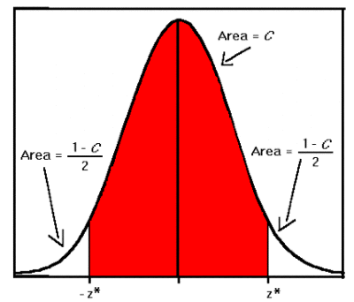
The length between the borders of the red area and the center is the loss value. The borders act as the stop loss and take profit value, as these are the value that the program predicts the price will fluctuate within.
Conclusion
Machine Learning and Stock Trading come hand in hand, as both are the prediction of complex patterns.
I hope that more people will use the Alpaca API and confidence intervals when it comes to algorithmic trading.
My links
If you want to see more of my content, click this link.
Alpaca does not prepare, edit, or endorse Third Party Content. Alpaca does not guarantee the accuracy, timeliness, completeness or usefulness of Third Party Content, and is not responsible or liable for any content, advertising, products, or other materials on or available from third party sites.
Brokerage services are provided by Alpaca Securities LLC ("Alpaca"), member FINRA/SIPC, a wholly-owned subsidiary of AlpacaDB, Inc. Technology and services are offered by AlpacaDB, Inc. This is not an offer, solicitation of an offer, or advice to buy or sell securities, or open a brokerage account in any jurisdiction where Alpaca is not registered (Alpaca is registered only in the United States).