In this post, we will demonstrate how to create a simple pipeline that uses Linear Regression to identify stock momentum, and filters stocks with the strongest momentum indicator. Then, analyzes going long and short on stocks from this signal. We will use Alphalens to analyze the quality of the Factor, then we will use pyfolio to analyze the returns from this factor. Eventually, we will create a simple zipline-trader algorithm that trades based on that signal and backtest it.
Table of Contents:
1). Loading the Data Bundle2). Calculating the Linear Regression Factor3). Creating the Pipeline4). Analyzing Performance Using Alphalens5). Working with pyfolio6). Backtesting our Alpha Factor7). Using pyfolio One More Time8). Final ThoughtsAll the data used in this post is from the Alpaca data API which could be obtained with a free account.
 Alpaca
Disclaimer: This is not a profitable strategy that you could deploy to live markets. It's written as an instructional post, showing the strengths of this framework and what you could do with it.
Now, let's get things started :)
Loading the Data Bundle
We use the Alpaca data service to create a data bundle that we feed into the zipline-trader's engine.
For a detailed explanation on how to connect the data to zipline-trader go to the zipline-trader docs: https://zipline-trader.readthedocs.io/en/latest/
Imports and Definitions:
import os
import pandas as pd
from datetime import timedelta
import zipline
from zipline.data import bundles
from zipline.utils.calendars import get_calendar
from zipline.pipeline.data import USEquityPricing
from zipline.pipeline.factors import CustomFactor
from zipline.research.utils import get_pricing, create_data_portal, create_pipeline_engine

os.environ['ZIPLINE_ROOT'] = os.path.join(os.getcwd(), '.zipline')

trading_calendar = get_calendar('NYSE')
bundle_name = 'alpaca_api'
start_date = pd.Timestamp('2015-12-31', tz='utc')
pipeline_start_date = start_date + timedelta(days=365*2)
while not trading_calendar.is_session(pipeline_start_date):
    pipeline_start_date += timedelta(days=1)
print(f"start date: {pipeline_start_date}")
end_date = pd.Timestamp('2020-12-28', tz='utc')
print(f"end date: {end_date}")
data_portal = create_data_portal(bundle_name, trading_calendar, start_date)
engine = create_pipeline_engine(bundle_name)
Calculating the Linear Regression Factor
This is a factor that runs a linear regression over one year of stock log returns and calculates a "slope" as our factor. It is based on the Alphalens example library.
import numpy as np
import pandas as pd
import scipy.stats as stats
from zipline.pipeline.factors import CustomFactor, Returns
from zipline.pipeline.data import USEquityPricing

def _slope(ts, x=None):
    if x is None:
        x = np.arange(len(ts))
    log_ts = np.log(ts)
    slope, intercept, r_value, p_value, std_err = stats.linregress(x, log_ts)
    return slope

class MyFactor(CustomFactor):
    """
    12 months Momentum
    Run a linear regression over one year (252 trading days) stocks log returns
    and the slope will be the factor value
    """
    inputs = [USEquityPricing.close]
    window_length = 252

    def compute(self, today, assets, out, close):
        x = np.arange(len(close))
        slope = np.apply_along_axis(_slope, 0, close, x.T)
        out[:] = slope
Creating the Pipeline
Let's create a pipeline that:
- Starts from our entire universe (S&P 500)
- Calculates AverageDollarVolume for the past 30 days, and selects the top 20 stocks.
- Calculate MyFactor for the 20 stocks selected in the previous step.
from zipline.pipeline.domain import US_EQUITIES
from zipline.pipeline.factors import AverageDollarVolume
from zipline.pipeline import Pipeline
from zipline.pipeline.classifiers.custom.sector import ZiplineTraderSector, SECTOR_LABELS

universe = AverageDollarVolume(window_length = 30).top(20)
my_factor = MyFactor()

pipeline = Pipeline(
    columns = {
            'MyFactor' : my_factor,
            'Sector' : ZiplineTraderSector(),
    }, domain=US_EQUITIES, screen=universe
)
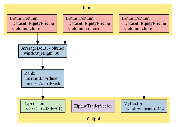
Plot the pipeline
We can plot our pipeline to get a visual sense of what the process does
pipeline.show_graph(format='png')
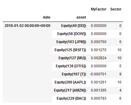
Run the Pipeline
# Run our pipeline for the given start and end dates
factors = engine.run_pipeline(pipeline, pipeline_start_date, end_date)

factors.head(),
Analyzing Performance Using Alphalens
Now we want to check if our factor has the potential for alpha generation. We will use Alphalens.
 quantopian
Data preparation
Alphalens input consists of two types of information: the factor values for the time period under analysis and the historical assets prices (or returns).
Alphalens doesn't need to know how the factor was computed, the historical factor values are enough. This is interesting because we can use the tool to evaluate factors for which we have the data but not the implementation details.
Alphalens requires that factor and price data follow a specific format and it provides a utility function, get_clean_factor_and_forward_returns, that accepts factor data, price data, and optionally group information (for example the sector groups, useful to perform sector specific analysis) and returns the data suitably formatted for Alphalens.
asset_list = factors.index.levels[1].unique()

prices = get_pricing(
        data_portal,
        trading_calendar,
        asset_list,
        pipeline_start_date,
        end_date)
prices.head(),
(                           Equity(0 [A])  Equity(1 [AAL])  Equity(2 [ABC])  \
 2018-01-03 00:00:00+00:00         69.340            52.12            94.42
 2018-01-04 00:00:00+00:00         68.805            52.45            94.17
 2018-01-05 00:00:00+00:00         69.890            52.65            95.33
 2018-01-08 00:00:00+00:00         70.060            52.11            96.90
 2018-01-09 00:00:00+00:00         71.780            52.07            97.52

                            Equity(3 [ABMD])  Equity(4 [ADP])  Equity(5 [AEE])  \
 2018-01-03 00:00:00+00:00            195.77           117.24            58.08
 2018-01-04 00:00:00+00:00            199.30           118.36            57.43
 2018-01-05 00:00:00+00:00            202.28           118.29            57.40
 2018-01-08 00:00:00+00:00            207.80           117.88            58.07
 2018-01-09 00:00:00+00:00            209.76           118.77            57.32

...

 [5 rows x 505 columns],)
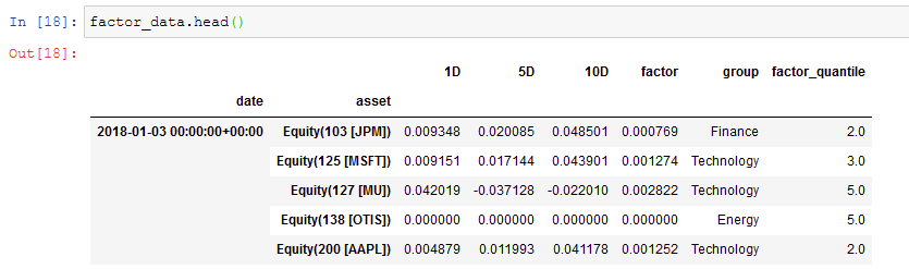
import alphalens as al
factor_data = al.utils.get_clean_factor_and_forward_returns(
        factor=factors["MyFactor"],
        prices=prices,
        quantiles=5,
        periods=[1, 5, 10],
        groupby=factors["Sector"],
        binning_by_group=True,
        groupby_labels=SECTOR_LABELS,
    max_loss=0.8)
Dropped 11.0% entries from factor data: 1.5% in forward returns computation and 9.6% in binning phase (set max_loss=0 to see potentially suppressed Exceptions).
max_loss is 80.0%, not exceeded: OK!
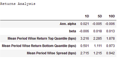
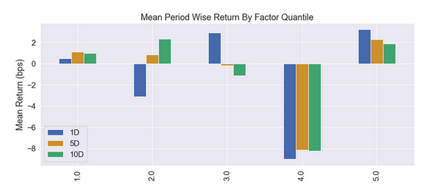
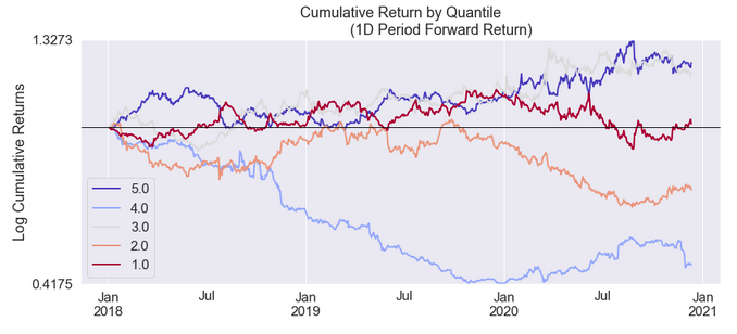
Running Alphalens
Once the factor data is ready, running Alphalens analysis is pretty simple and it consists of one function call that generates the factor report (statistical information and plots). Please remember that it is possible to use the help python built-in function to view the details of a function.
al.tears.create_full_tear_sheet(factor_data, long_short=True, group_neutral=True, by_group=True)
A Part of the Full Report below edited down for readability
These reports are also available
al.tears.create_returns_tear_sheet(factor_data,
                                   long_short=True,
                                   group_neutral=False,
                                   by_group=False)

al.tears.create_information_tear_sheet(factor_data,
                                       group_neutral=False,
                                       by_group=False)

al.tears.create_turnover_tear_sheet(factor_data)

al.tears.create_event_returns_tear_sheet(factor_data, prices,
                                         avgretplot=(5, 15),
                                         long_short=True,
                                         group_neutral=False,
                                         std_bar=True,
                                         by_group=False)
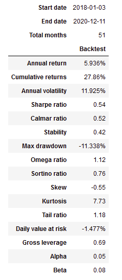
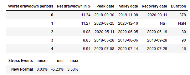
Working with pyfolio
We could use pyfolio to analyze the returns as if it was generated by a backtest, like so
pf_returns, pf_positions, pf_benchmark = \
    al.performance.create_pyfolio_input(factor_data,
                                        period='1D',
                                        capital=100000,
                                        long_short=True,
                                        group_neutral=False,
                                        equal_weight=True,
                                        quantiles=[1,5],
                                        groups=None,
                                        benchmark_period='1D')
import pyfolio as pf
pf.tears.create_full_tear_sheet(pf_returns,
                                positions=pf_positions,
                                benchmark_rets=pf_benchmark,
                                hide_positions=True)
A Part of the Full Report below edited down for readability
Backtesting our Alpha Factor
Let's now create a simple algorithm that wraps our pipeline and backtest it against our data bundle as if we run it in a live market. This is more realistic than what we just did with pyfolio since we do not run a factor in live trading. There are a lot of moving parts and we need to wrap it in a logic that works under the market conditions.
Our simple algorithm will:
- Run the pipeline we created daily.
- Longs the top 5 stocks, Shorts the bottom 5.
Our zipline-trader Algorithm
from zipline.research.utils import DATE, get_benchmark
from zipline.api import order_target, record, symbol
import matplotlib.pyplot as plt
from zipline.api import (
    attach_pipeline,
    order_target_percent,
    pipeline_output,
    record,
    schedule_function,
    date_rules,
    time_rules
)

def initialize(context):
    attach_pipeline(pipeline, 'my_pipeline', chunks=1)

def rebalance(context, data):
    my_pipe = context.pipeline_data.sort_values('MyFactor', ascending=False).MyFactor
    for equity in my_pipe[:5].index:
        if equity not in context.get_open_orders():
            order_target_percent(equity, 0.2)
    for equity in my_pipe[-5:].index:
        if equity not in context.get_open_orders():
            order_target_percent(equity, -0.2)

def close_positions(context, data):
    my_pipe = context.pipeline_data.sort_values('MyFactor', ascending=False).MyFactor
    for equity in context.portfolio.positions:
        if equity not in my_pipe[:5] and equity not in my_pipe[-5:]:
            if equity not in context.get_open_orders():
                order_target(equity, 0)

def handle_data(context, data):
    pass

def before_trading_start(context, data):
    context.pipeline_data = pipeline_output('my_pipeline')
    schedule_function(rebalance, date_rules.every_day(), time_rules.market_open(minutes=10))
    schedule_function(close_positions, date_rules.every_day(), time_rules.market_open(minutes=5))
Backtest Execution
Let's now run our backtest for the year 2020
import pandas as pd
from datetime import datetime
import pytz

from zipline import run_algorithm

start = pd.Timestamp(datetime(2020, 1, 1, tzinfo=pytz.UTC))
end = pd.Timestamp(datetime(2020, 12, 1, tzinfo=pytz.UTC))

r = run_algorithm(start=start,
                  end=end,
                  initialize=initialize,
                  capital_base=100000,
                  handle_data=handle_data,
                  benchmark_returns=get_benchmark(symbol="SPY",
                  start=start.date().isoformat(),
                  end=end.date().isoformat()),
                  bundle='alpaca_api',
                  broker=None,
                  state_filename="./demo.state",
                  trading_calendar=trading_calendar,
                  before_trading_start=before_trading_start,
                  data_frequency='daily'
                  )
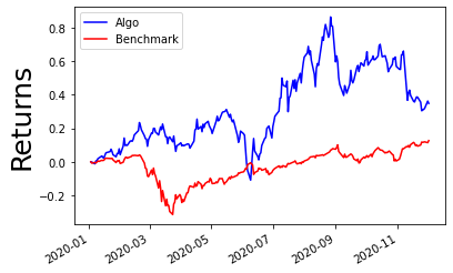
r.algorithm_period_return.plot(color='blue')
r.benchmark_period_return.plot(color='red')
plt.legend(['Algo', 'Benchmark'])
plt.ylabel("Returns", color='black', size=25)
Using pyfolio One More Time
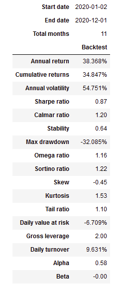
We can use pyfolio once again to analyze the performance of the backtest we just execute
import pyfolio as pf

returns, positions, transactions = pf.utils.extract_rets_pos_txn_from_zipline(r)
benchmark_returns = r.benchmark_period_return
import empyrical
print(f"returns sharp ratio: {empyrical.sharpe_ratio(returns):.2}")
print("beta ratio: {:.2}".format(empyrical.beta(returns, benchmark_returns)))
print("alpha ratio: {:.2}".format(empyrical.alpha(returns, benchmark_returns)))
returns sharp ratio: 0.87
beta ratio: -0.0032
alpha ratio: 0.58
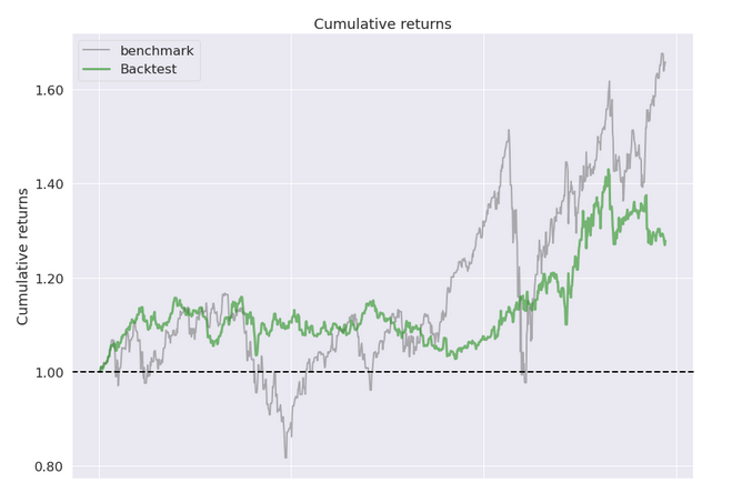
pf.create_returns_tear_sheet(returns,
                             positions=positions,
                             transactions=transactions,
                             benchmark_rets=benchmark_returns)
A Part of the Full Report below edited down for readability
Final Thoughts
All and all we got pretty good results with positive returns. We did better than our benchmark (SPY) for the year 2020. So it could be a basis for creating something more robust.
What next?
- We had significant drawdowns, one could minimize these.
- One can backtest during a much longer period.
- One can optimize the pipeline. The above example is just a simple setup, definitely not the optimized setup so different parameters would create different results.
- One could implement this in paper trading. While backtests are good, but it is important to see what happens in real time.
- The wrapping algorithm is extremely simplified, much more work could be done there.
- One could make the algorithm sector neutral, or maybe even find better responding sectors.
To learn more about this framework and how to install and set it up, go to the docs: https://zipline-trader.readthedocs.io/en/latest/
Used python libraries
shlomikushchi quantopianquantopianscipy
 pandas-dev
 numpy
numpy
Technology and services are offered by AlpacaDB, Inc. Brokerage services are provided by Alpaca Securities LLC (alpaca.markets), member FINRA/SIPC. Alpaca Securities LLC is a wholly-owned subsidiary of AlpacaDB, Inc.