Backtesting 0DTE Options: The Complete Guide to Strategy, Setup & Performance

Previously, we explored what 0DTE options are and explained how to trade them using Alpaca’s Trading API in Python, covering both the advantages and challenges of 0DTE strategies. We also discussed how option Greeks like theta and delta impact these trades. In this guide, we’ll focus on how to backtest a 0DTE bull put spread strategy and evaluate its performance using Alpaca’s Trading API and the Databento API.

Overview: How to Backtest 0DTE Bull Put Spread Options Strategies Using Alpaca and Databento

Before diving into the code sections, it’s important to first understand the overall structure of the backtesting process and how the algorithm can be configured.

You can also refer to the README.md file in the GitHub repository for more details on the backtesting logic.

Bull Put Spread Strategy Overview

• Sell a higher-strike put (collect premium)
• Buy a lower-strike put (limit risk)
• Net result: Receive credit upfront, profit if underlying stays above short strike
• Learn more about the bull put spread strategy

How the Selection Process Works 

The process used in this notebook scans through historical market data chronologically at one-minute intervals to find the first valid option pair that meets our trading criteria, holds it until an exit condition is met, then repeats every minute:

1. Delta-based Selection
   1. Short Put: Higher delta (closer to ATM) - generates premium income
   2. Long Put: Lower delta (further OTM) - provides downside protection
2. Spread Width Validation
   1. Ensures risk/reward ratio stays within acceptable bounds
   2. Configurable range (default: $2–$4) balances premium vs. risk
3. Chronological Priority
   1. Selects the first valid pair found in time sequence
   2. Mimics real-world trading where timing matters

Environment Configuration 

• The notebook automatically detects whether it's running in Google Colab or not
• API keys are loaded differently based on the environment:
  • Google Colab: Uses Colab's Secrets feature (set keys in the left sidebar)
  • Jupyter Notebook (e.g. VS Code, PyCharm): Uses environment variables from a `.env` file
  • Required API Keys:
    • `ALPACA_API_KEY` and `ALPACA_SECRET_KEY` from your Alpaca dashboard
    • `DATABENTO_API_KEY` from your Databento dashboard

Data Sources

Dual API Integration for Comprehensive Market Data

• Alpaca Trading API: Stock daily bars + 1-minute intraday data
• Databento API with OPRA Standard plan: Options 1-minute tick data with bid/ask spreads

This combination provides both the underlying stock context and detailed options pricing needed for accurate 0DTE backtesting, leveraging each platform's strengths.

If you want to know more about how to code alpaca-py, check out the following resources:

• Alpaca-py GitHub Page
• Alpaca-py Documentation
• API Reference of Alpaca APIs

Note: This backtest requires both Alpaca’s Trading API and Databento's Historical API. In this demo, we use OPRA (Options Price Reporting Authority) equity options data from Databento, which can be accessed with usage-based pricing or through a subscription plan. Please review the following Databento resources below:

• Quickstart (Set up Databento)
• OPRA Standard plan details
• Equity options: Introduction

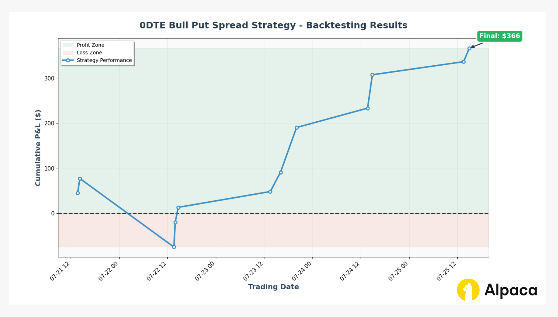
Here’s a preview of the cumulative P&L line chart that this backtest will ultimately generate.

Backtesting the Options Strategy with Alpaca's Trading API and Databento API

Step 0: Installing Dependencies and Importing Libraries

We’ll use the uv Python package manager to install all the necessary packages before starting the backtesting process.

!uv pip install databento alpaca-py python-dotenv pandas numpy scipy matplotlib jupyter ipykernel

import os
import sys
from datetime import date, datetime, time, timedelta
from typing import Dict, List, Optional, Tuple
from zoneinfo import ZoneInfo

import databento as db
import matplotlib.pyplot as plt
import numpy as np
import pandas as pd
from dotenv import load_dotenv
from scipy.optimize import brentq
from scipy.stats import norm

from alpaca.data.historical.option import OptionHistoricalDataClient
from alpaca.data.historical.stock import StockHistoricalDataClient
from alpaca.data.requests import StockBarsRequest
from alpaca.data.timeframe import TimeFrame, TimeFrameUnit
from alpaca.trading.client import TradingClient
from alpaca.trading.enums import ContractType
from alpaca.trading.requests import GetCalendarRequest

Step 1: Setting UP the Environment and Trade Parameters

This section sets up the environment configuration keys for each working environment (flexibly adjusting for Google Colab or local IDEs), initializes Alpaca clients and the Databento client, and defines key parameters like date information and key algorithm thresholds, which users can adjust.

The environment configuration automatically detects whether it's running in Google Colab or a local IDE and loads API keys accordingly

• Alpaca clients are initialized for trading, options historical data, and stock data
• Databento client is initialized for options tick data
• Key parameters include date ranges, delta thresholds, stop loss settings, and profit targets

if "google.colab" in sys.modules:
    # In Google Colab environment, we will fetch API keys from Secrets.
    # Please set ALPACA_API_KEY, ALPACA_SECRET_KEY, DATABENTO_API_KEY in Google Colab's Secrets from the left sidebar
    from google.colab import userdata

    ALPACA_API_KEY = userdata.get("ALPACA_API_KEY")
    ALPACA_SECRET_KEY = userdata.get("ALPACA_SECRET_KEY")
    DATABENTO_API_KEY = userdata.get("DATABENTO_API_KEY")
else:
    # Please safely store your API keys and never commit them to the repository (use .gitignore)
    # Load environment variables from environment file (e.g., .env)
    load_dotenv()
    # API credentials for Alpaca's Trading API and Databento API
    ALPACA_API_KEY = os.environ.get("ALPACA_API_KEY")
    ALPACA_SECRET_KEY = os.environ.get("ALPACA_SECRET_KEY")
    DATABENTO_API_KEY = os.getenv("DATABENTO_API_KEY")

## We use paper environment for this example
ALPACA_PAPER_TRADE = True  # Please do not modify this. This example is for paper trading only.


# Below are the variables for development this documents (Please do not change these variables)
TRADE_API_URL = None
TRADE_API_WSS = None
DATA_API_URL = None
OPTION_STREAM_DATA_WSS = None

# Signed Alpaca clients
from alpaca import __version__ as alpacapy_version

class _ClientMixin:
    def _get_default_headers(self):
        headers = self._get_auth_headers()
        headers["User-Agent"] = "APCA-PY/" + alpacapy_version + "-ZERO-DTE-NOTEBOOK"
        return headers

class TradingClientSigned(_ClientMixin, TradingClient): pass
class OptionHistoricalDataClientSigned(_ClientMixin, OptionHistoricalDataClient): pass
class StockHistoricalDataClientSigned(_ClientMixin, StockHistoricalDataClient): pass

We initialize Alpaca’s clients.

# Initialize Alpaca clients
trade_client = TradingClientSigned(api_key=ALPACA_API_KEY, secret_key=ALPACA_SECRET_KEY, paper=ALPACA_PAPER_TRADE)
option_historical_data_client = OptionHistoricalDataClientSigned(api_key=ALPACA_API_KEY, secret_key=ALPACA_SECRET_KEY)
stock_data_client = StockHistoricalDataClientSigned(api_key=ALPACA_API_KEY, secret_key=ALPACA_SECRET_KEY)

We also initialize the Databento historical client as well. Please check out the Databento API reference - Historical for further information.

# Initialize Databento client
databento_client = db.Historical(DATABENTO_API_KEY)

For an algorithmic 0DTE bull put spread, selecting the right strategy inputs is crucial to managing risk and reward logics effectively. These inputs allow each trade to meet predetermined strategy criteria.

# Underlying symbol
underlying_symbol = "SPY"

# Risk free rate for the options greeks and IV calculations
RISK_FREE_RATE = 0.01

# Set the timezone
NY_TZ = ZoneInfo("America/New_York")

# Get current date in US/Eastern timezone
today = datetime.now(NY_TZ).date()
start_date = today - timedelta(days=10)  # Start of backtesting period: 10 trading days of 0DTE strategy data
end_date = today - timedelta(days=2)  # End of backtesting period: excludes recent data

# Set buffer percentage for the strike price range (default: ±5%)
BUFFER_PCT = 0.05

# Define delta thresholds
SHORT_PUT_DELTA_RANGE = (-0.60, -0.20)  # Short put selection: delta between -0.60 to -0.20 for bull put spread
LONG_PUT_DELTA_RANGE = (-0.40, -0.20)  # Long put selection: delta between -0.40 to -0.20 for bull put spread

# Set stop loss threshold threshold (2 times of the initial delta)
DELTA_STOP_LOSS_THRES = 2

# Set target profit and stop-loss levels (50% of the initial credit)
TARGET_STOP_LOSS_PERCENTAGE = 0.5

Step 2: Getting Historical Stock Daily Bar Data

We define daily price boundaries with a small buffer (BUFFER_PCT, default: ±5%) around the high and low prices. This allows us to focus on realistic strike prices near the market price (where bull put spreads are typically placed) rather than downloading all available one-minute option contracts and equities bars data.

• The `get_daily_stock_bars_df` function fetches daily price bars for the underlying stock (e.g., SPY) within the specified date range using Alpaca's API.
• The function also retrieves market calendar data to get accurate market close times, with an additional 15 minutes added for symbols that have the 'options_late_close' attribute (like SPY).

Please note that we are using SPY as an example and it should not be considered investment advice.

def get_daily_stock_bars_df(
    symbol: str, start_date: date, end_date: date
) -> pd.DataFrame:
    """
    Retrieve daily stock bars and replace timestamps with actual market close times.

    Used to establish daily high/low price boundaries for option strike selection.
    Gets actual market hours from Alpaca's trading calendar to handle early/late market closes.
    Adds 15 minutes to expiration time for symbols with 'options_late_close' attribute.

    Args:
        symbol (str): Stock ticker symbol (e.g., 'SPY')
        start_date (date): Start date for data retrieval
        end_date (date): End date for data retrieval

    Returns:
        pd.DataFrame: Daily OHLCV data with expiration_datetime index containing
                     actual market close times from Alpaca's trading calendar
    """

    req = StockBarsRequest(
        symbol_or_symbols=symbol,
        timeframe=TimeFrame(amount=1, unit=TimeFrameUnit.Day),
        start=start_date,
        end=end_date,
    )
    res = stock_data_client.get_stock_bars(req)
    # Convert the response to DataFrame
    df = res.df

    # Get market calendar for the same date range
    calendar_request = GetCalendarRequest(start=start_date, end=end_date)
    calendar = trade_client.get_calendar(calendar_request)

    # Check if symbol has options_late_close attribute
    asset_info = trade_client.get_asset(symbol_or_asset_id=symbol)
    extra_minutes = 15 if "options_late_close" in asset_info.attributes else 0

    # Create market close lookup with conditional 15-minute addition for options_late_close assets
    market_close_lookup = {
        cal.date: cal.close.replace(tzinfo=NY_TZ) + timedelta(minutes=extra_minutes)
        for cal in calendar
    }

    # Replace timestamp with actual market close datetime after reformatting the dataframe
    df = df.reset_index().drop(columns=["symbol"])
    df["expiration_datetime"] = df["timestamp"].dt.date.map(market_close_lookup.get)
    df = df.drop(columns=["timestamp"]).set_index("expiration_datetime").sort_index()

    return df

We run the `get_daily_stock_bars_df` function to retrieve the daily stock bars for the underlying symbol and save the result as `stock_bars_data`.

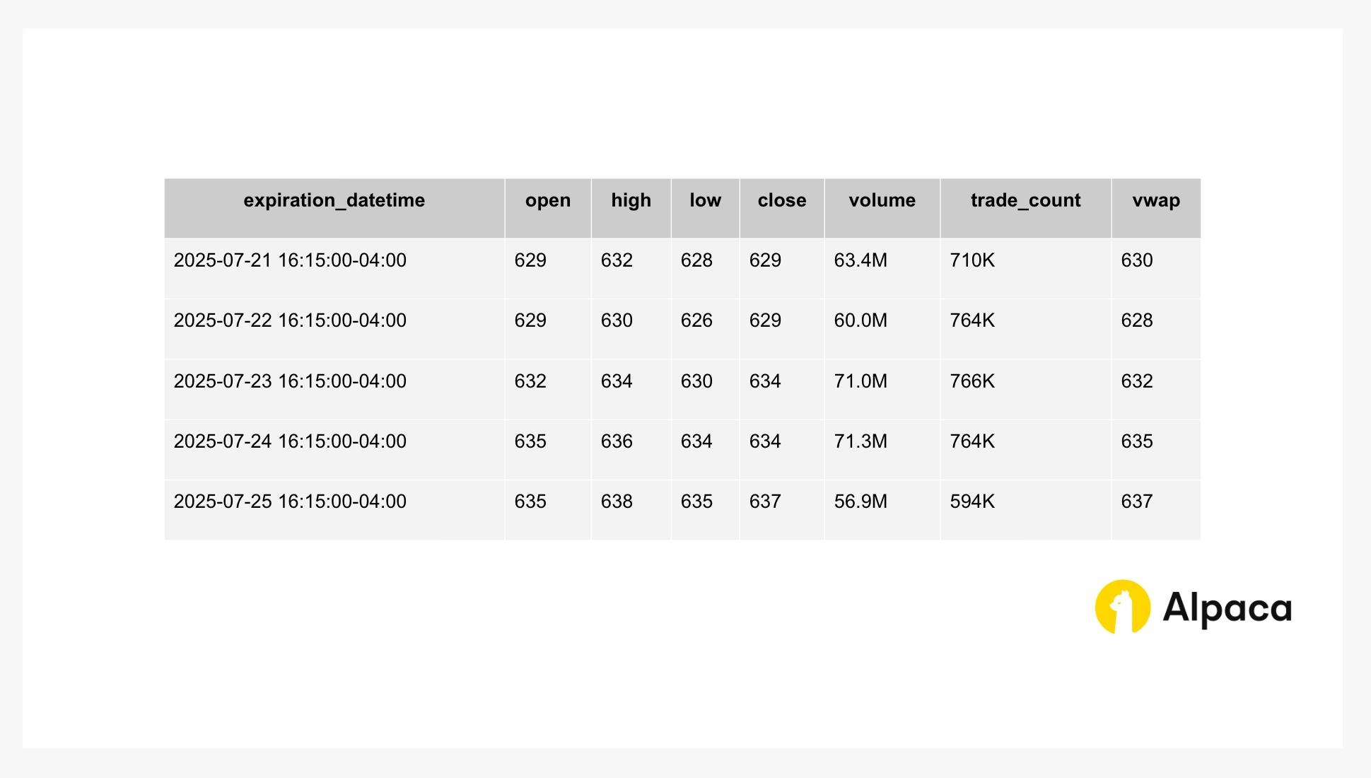
stock_bars_data = get_daily_stock_bars_df(symbol=underlying_symbol, start_date=start_date, end_date=end_date)

Running the code below will display data like the table.

stock_bars_data

The code would return the output shown below.

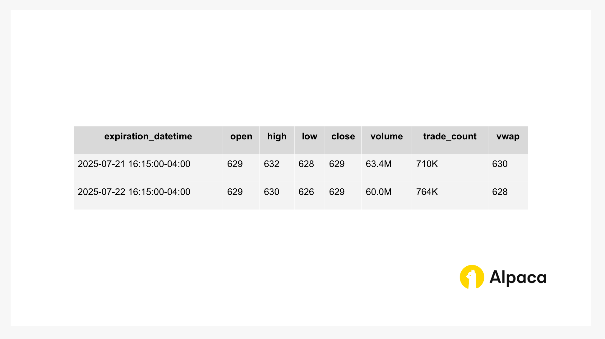
You can also get the first 2 rows of the stock bars data

stock_bars_data.head(2)

The code would return the output shown below.

Step 3: Retrieving Historical Minute-by-Minute Stock and Options Data by Expiration

This section generates the universe of relevant put option contracts for backtesting by creating option symbols within a realistic strike price range (±5% buffer around daily high/low prices) and grouping by expiration date based on daily stock bars data. This targeted approach ensures we only fetch option data that traders would realistically consider for bull put spreads, rather than downloading all available contracts.

The `calculate_strike_price_range` calculates the range of option strike prices to consider based on the stock's daily high/low prices with a buffer percentage.

def calculate_strike_price_range(
    high_price: float, low_price: float, buffer_pct: float = 0.05
) -> Tuple[float, float]:
    """
    Calculate strike price boundaries with buffer around daily high/low prices.

    Args:
        high_price: Daily high price
        low_price: Daily low price
        buffer_pct: Percentage buffer to expand range (default 5%)

    Returns:
        Tuple[float, float]: (min_strike, max_strike) boundaries
    """
    min_strike = low_price * (1 - buffer_pct)
    max_strike = high_price * (1 + buffer_pct)

    return min_strike, max_strike

Show only the first row.

# Set pandas to display numbers in decimal format instead of scientific notation
pd.set_option('display.float_format', '{:.2f}'.format)

first_row = stock_bars_data.iloc[0]
print(first_row)
min_strike, max_strike = calculate_strike_price_range(
    first_row["high"], first_row["low"], buffer_pct=BUFFER_PCT
)
print("--------------------------------")

print(
    f"{first_row.name.date()}: min_strike with 5% buffer=${min_strike:.2f}, max_strike with 5% buffer=${max_strike:.2f}"
)

The code would return the output shown below.

open               628.77
high               631.54
low                628.34
close              628.77
volume        63374984.00
trade_count     709907.00
vwap               630.17
Name: 2025-07-21 16:15:00-04:00, dtype: float64
--------------------------------
2025-07-21: min_strike with 5% buffer=$596.92, max_strike with 5% buffer=$663.12

The `generate_put_option_symbols` uses the strike price range to generate standardized option symbol strings for put options within the specified range.

def generate_put_option_symbols(
    underlying: str,
    expiration_datetime: datetime,
    min_strike: float,
    max_strike: float,
    strike_increment: float = 1,
) -> List[str]:
    """
    Generate put option symbols for the given parameters.

    Uses ceiling function to round min_strike UP to nearest whole dollar
    (e.g., $590.96 becomes $591) since options usually trade at integer strikes.

    Args:
        underlying: Underlying symbol (e.g., 'SPY')
        expiration_datetime: Option expiration datetime
        min_strike: Minimum strike price
        max_strike: Maximum strike price
        strike_increment: Strike price increment (default 1)

    Returns:
        List[str]: Formatted option symbols (e.g., 'SPY250616P00571000')
    """
    option_symbols = []

    # Format expiration datetime as date: YYMMDD
    expiration_date = expiration_datetime.date()
    exp_str = expiration_date.strftime("%y%m%d")

    # Generate strikes in increments (rounds UP to the nearest integer)
    current_strike = np.ceil(min_strike / strike_increment) * strike_increment

    while current_strike <= max_strike:
        # Format strike price as 8-digit integer (multiply by 1000)
        strike_formatted = f"{int(current_strike * 1000):08d}"

        # Create option symbol: SPY + YYMMDD + P + 8-digit strike
        option_symbol = f"{underlying}{exp_str}P{strike_formatted}"
        option_symbols.append(option_symbol)

        current_strike += strike_increment

    return option_symbols

The `collect_option_symbols_by_expiration` creates a list of all relevant option symbols grouped by expiration date for simulating the 0DTE strategy.

def collect_option_symbols_by_expiration(
    stock_bars_data: pd.DataFrame, underlying_symbol: str, buffer_pct: float
) -> Dict[pd.Timestamp, List[str]]:
    """
    Collect option symbols grouped by expiration datetime for 0DTE backtesting.

    For each trading day in the stock bars data, generates put option symbols
    within a realistic strike range and groups them by expiration date.

    Args:
        stock_bars_data: DataFrame containing daily OHLCV data with timestamp index
        underlying_symbol: Stock symbol (e.g., 'SPY') for option generation
        buffer_pct: Buffer percentage to expand strike range around daily high/low

    Returns:
        Dict[pd.Timestamp, List[str]]: Dictionary mapping expiration datetime (e.g., Timestamp('2025-07-21 16:00:00'))
                                       to lists of option symbols for that date
    """
    # Collect all symbols
    option_symbols_by_expiration = {}

    for index, row in stock_bars_data.iterrows():
        min_strike, max_strike = calculate_strike_price_range(
            row["high"], row["low"], buffer_pct=buffer_pct
        )

        option_symbols = generate_put_option_symbols(
            underlying_symbol,
            expiration_datetime=index,
            min_strike=min_strike,
            max_strike=max_strike,
            strike_increment=1,
        )

        # Group symbols by expiration date
        if index not in option_symbols_by_expiration:
            option_symbols_by_expiration[index] = []

        option_symbols_by_expiration[index].extend(option_symbols)

    return option_symbols_by_expiration

option_symbols_by_expiration = collect_option_symbols_by_expiration(
    stock_bars_data, underlying_symbol, buffer_pct=BUFFER_PCT
)

This code displays expiration time, total count, and first 5 symbols as a sample.

timestamp = list(option_symbols_by_expiration.keys())[0]
symbols = list(option_symbols_by_expiration.values())[0]

print(f"Expiration: {timestamp}")
print(f"Total symbols: {len(symbols)}")
print(f"Sample symbols: {symbols[:5]}")

The code would return the output shown below.

Expiration: 2025-07-21 16:15:00-04:00
Total symbols: 67
Sample symbols: ['SPY250721P00597000', 'SPY250721P00598000', 'SPY250721P00599000', 'SPY250721P00600000', 'SPY250721P00601000']

This code shows just the keys (dates) to understand the structure.

keys = list(option_symbols_by_expiration.keys())
keys

The code would return the output shown below.

[Timestamp('2025-07-21 16:15:00-0400', tz='America/New_York'),
 Timestamp('2025-07-22 16:15:00-0400', tz='America/New_York'),
 Timestamp('2025-07-23 16:15:00-0400', tz='America/New_York'),
 Timestamp('2025-07-24 16:15:00-0400', tz='America/New_York'),
 Timestamp('2025-07-25 16:15:00-0400', tz='America/New_York')]

This code displays the maximum and minimum strike price ranges for option data, as well as the first two and last two option symbols to compare calculated vs generated strike ranges.

# Compare calculated vs generated strike ranges. You can see that the generated strike ranges are within the calculated range.
first_day = stock_bars_data.head(1).iloc[0]
calc_min, calc_max = (
    first_day["low"] * (1 - BUFFER_PCT),
    first_day["high"] * (1 + BUFFER_PCT),
)
print(f"Calculated range with 5% buffer for option symbols for the first day: ${calc_min:.2f} - ${calc_max:.2f}")

symbols = option_symbols_by_expiration[keys[0]]  # Show the first expiration date's option symbols
(symbols[:2] + ["..."] + symbols[-2:])  # Show first 2 and last 2 option symbols to see the strike range

The code would return the output shown below.

Calculated range with 5% buffer for option symbols for the first day: $596.92 - $663.12

['SPY250721P00597000',
 'SPY250721P00598000',
 '...',
 'SPY250721P00662000',
 'SPY250721P00663000']

The `extract_strike_price_from_symbol` function is a helper function that extracts the strike price from each option symbol and is incorporated into the `get_historical_stock_and_option_data` function.

def extract_strike_price_from_symbol(symbol: str) -> float:
    """
    Extract strike price from option symbol.
    Converts last 8 digits of option symbol to strike price by dividing by 1000.

    Args:
        symbol: Option symbol (e.g., 'SPY250616P00571000')

    Returns:
        float: Strike price (e.g., 571.0) or 0.0 if invalid format
    """
    # Option symbols typically have format: TICKER + YYMMDD + (C/P) + 8-digit strike price
    # The last 8 digits represent strike price * 1000
    try:
        # Extract the last 8 digits and convert to strike price
        strike_str = symbol[-8:]
        strike_price = float(strike_str) / 1000.0
        return strike_price
    except (ValueError, IndexError):
        print(f"Warning: Could not extract strike price from symbol {symbol}")
        return 0.0

The `get_historical_stock_and_option_data` function uses the collection of all relevant option symbols grouped by expiration timestamp from the `collect_option_symbols_by_expiration` function and retrieves minute-by-minute market data for both stock and options using Alpaca and Databento APIs, providing the data needed for realistic backtesting.

def get_historical_stock_and_option_data(
    option_symbols_by_expiration: Dict[pd.Timestamp, List[str]], underlying_symbol: str
) -> pd.DataFrame:
    """
    Get combined option and stock data as a DataFrame.
    Returns options data with stock close prices merged by timestamp for easier inspection.

    Args:
        option_symbols_by_expiration: Dictionary mapping dates to option symbol lists
        underlying_symbol: Stock symbol for underlying asset

    Returns:
        pd.DataFrame: Combined options and stock data with renamed columns
    """
    all_data_frames = []

    for expiration_datetime, symbols_list in option_symbols_by_expiration.items():
        # Create start datetime at 9:30 AM for the same date
        start_datetime = expiration_datetime.replace(hour=9, minute=30, second=0, microsecond=0)
        # Use expiration_datetime directly as end_datetime (already contains actual market close)
        end_datetime = expiration_datetime

        # Get stock bar data (1 minute interval) for the specified underlying symbol
        req = StockBarsRequest(
            symbol_or_symbols=underlying_symbol,
            timeframe=TimeFrame(amount=1, unit=TimeFrameUnit.Minute),
            start=start_datetime,
            end=end_datetime,
        )
        stock_res = stock_data_client.get_stock_bars(req)

        # Create a dictionary of stock close prices by timestamp for quick lookup
        stock_close_by_timestamp = {}
        if underlying_symbol in stock_res.data:
            for bar in stock_res.data[underlying_symbol]:
                stock_close_by_timestamp[bar.timestamp] = bar.close
            print(f"Retrieved 1-minute stock bars for {underlying_symbol} on {expiration_datetime.date()}: {len(stock_res.data[underlying_symbol])} total bars from Alpaca Trading API")

            # Transform options symbols to format required by databento (add spaces)
            formatted_option_symbols = [f"{symbol[:3]}   {symbol[3:]}" for symbol in symbols_list]

            # Get all options strikes available for this date using databento client
            available_options_df = databento_client.timeseries.get_range(
                dataset="OPRA.PILLAR",
                schema="definition",
                symbols=f"{underlying_symbol}.OPT",
                stype_in="parent",
                start=start_datetime.date(),
            ).to_df()

            # Filter for strikes that are active
            filtered_option_symbols = [
                sym for sym in formatted_option_symbols
                if sym in available_options_df["raw_symbol"].to_list()
            ]

            # Get option tick data using databento client
            option_df = databento_client.timeseries.get_range(
                dataset="OPRA.PILLAR",
                schema="cbbo-1m",
                symbols=filtered_option_symbols,
                start=start_datetime,
                end=end_datetime,
            ).to_df()

            if not option_df.empty:
                # Add derived columns to option_df
                option_df["option_symbol"] = option_df["symbol"].str.replace(" ", "")
                option_df["strike_price"] = option_df["option_symbol"].apply(extract_strike_price_from_symbol)
                option_df["midpoint"] = (option_df["bid_px_00"] + option_df["ask_px_00"]) / 2
                option_df["expiry"] = end_datetime.astimezone(ZoneInfo("UTC"))

                # Map stock close prices using timestamp lookup (handles one-to-many correctly)
                option_df["underlying_close"] = option_df.index.map(stock_close_by_timestamp)

                # Select and rename columns as needed
                final_df = option_df[
                    [
                        "option_symbol",
                        "strike_price",
                        "price",
                        "bid_px_00",
                        "ask_px_00",
                        "midpoint",
                        "bid_sz_00",
                        "ask_sz_00",
                        "expiry",
                        "underlying_close",
                    ]
                ].rename(
                    columns={
                        "price": "close",
                        "bid_px_00": "bid",
                        "ask_px_00": "ask",
                        "bid_sz_00": "bid_size",
                        "ask_sz_00": "ask_size",
                    }
                )

                # Reset index to make timestamp a column and rename it
                final_df.reset_index(inplace=True)
                final_df.rename(columns={"ts_recv": "timestamp"}, inplace=True)

                all_data_frames.append(final_df)
                print(f"Retrieved 1-minute option tick data for {len(formatted_option_symbols)} option symbols on {expiration_datetime.date()}: {len(option_df)} total rows from Databento API")
            else:
                print(f"No data found for options symbols: {formatted_option_symbols}")

    # Combine all DataFrames
    if all_data_frames:
        result_df = pd.concat(all_data_frames, ignore_index=True)
        return result_df.sort_values("timestamp").reset_index(drop=True)
    else:
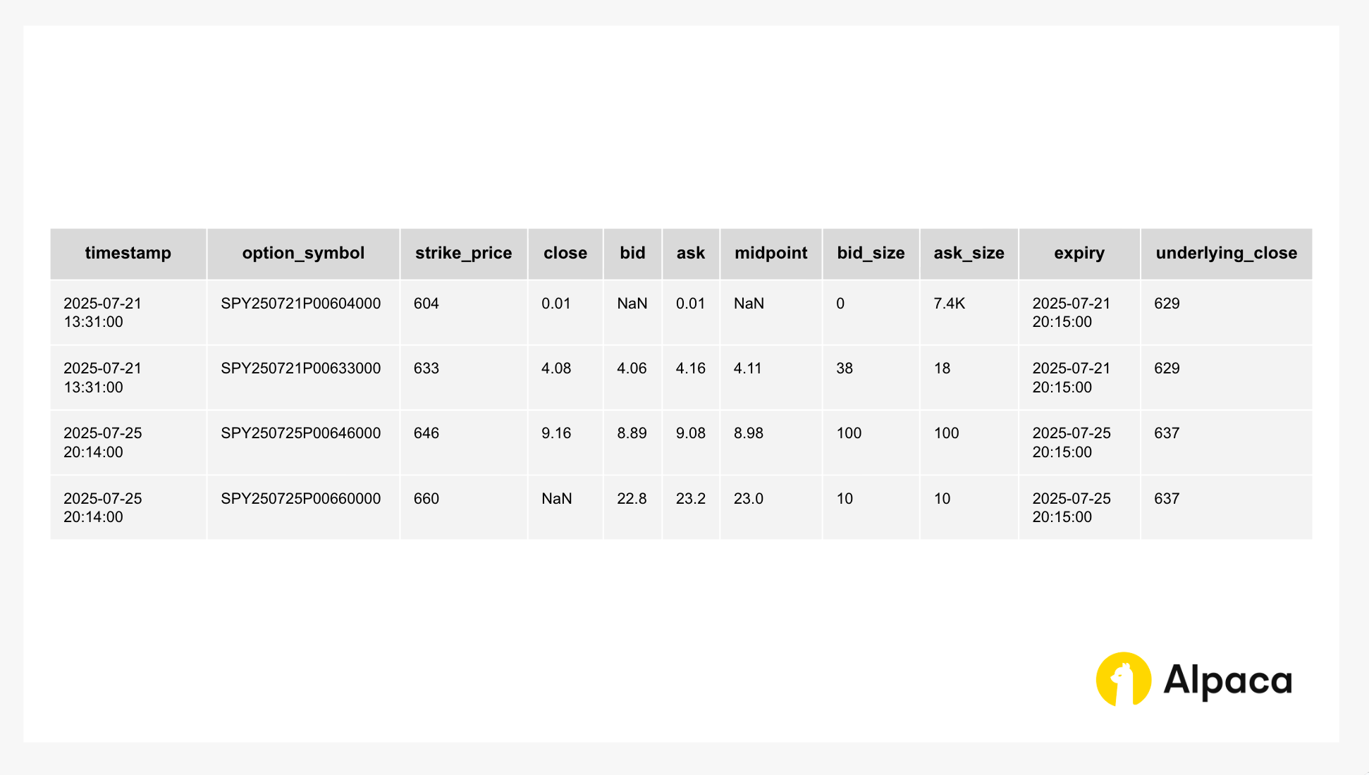
        return pd.DataFrame()

The option_df (option tick data retrieved via Databento's API) within the `get_historical_stock_and_option_data` function looks like this. This example only shows relevant columns, while others have been omitted.

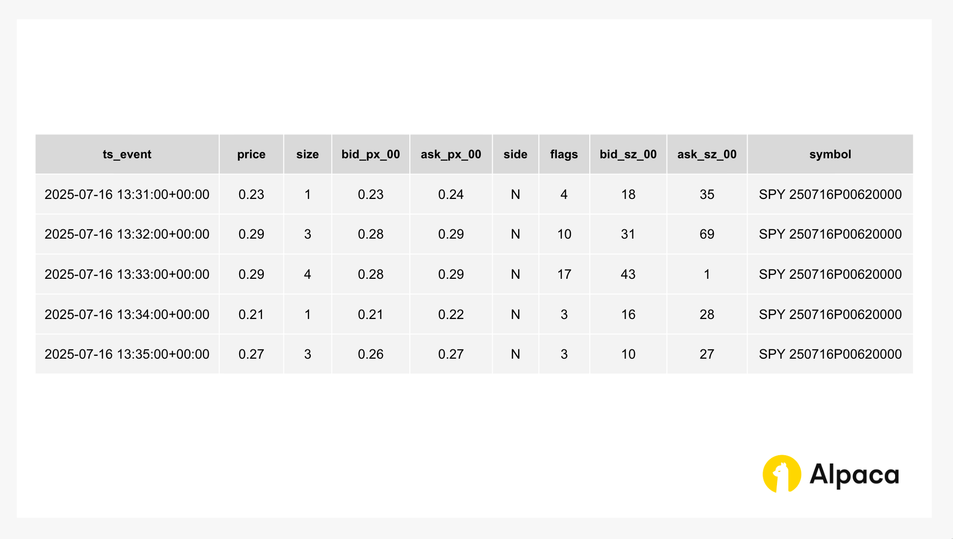
When you run the code below, you would receive something similar to the following output.

historical_stock_and_option_data = get_historical_stock_and_option_data(
    option_symbols_by_expiration, underlying_symbol
)

The code would return the output shown below.

Retrieved 1-minute stock bars for SPY on 2025-07-21: 406 total bars from Alpaca Trading API
Retrieved 1-minute option tick data for 67 option symbols on 2025-07-21: 22533 total rows from Databento API
...

Now you can get the historical data of both stock and option data. Here, we simply display the first 2 and last 2 rows of the output.

# Show first 2 and last 2 rows of the stock_option_historical_data_by_timestamp
pd.concat(
    [historical_stock_and_option_data.head(2), historical_stock_and_option_data.tail(2)]
)

The code would return the output shown below.

Step 4: Implementing Options Greeks and IV Calculations from Historical Option Bars

Calculate delta and implied volatility (IV) for each 1-minute option tick to determine which options qualify for our bull put spread. Delta measures price sensitivity to stock movements, while the IV helps us determine if the option is fairly priced. Both help us select appropriate short puts (higher delta) and long puts (lower delta) for the strategy.

The `calculate_implied_volatility` function estimates the IV of an option by solving for the volatility that matches the observed option price, using the Black-Scholes model. It handles edge cases where the option price is close to intrinsic value by returning a near-zero volatility.

# Calculate implied volatility
def calculate_implied_volatility(
    option_price: float, S: float, K: float, T: float, r: float, option_type: str
) -> Optional[float]:
    """
    Calculate implied volatility using the Black-Scholes model.

    Args:
        option_price: Market price of the option
        S: Current stock price (underlying asset price)
        K: Strike price of the option
        T: Time to expiration in years
        r: Risk-free interest rate
        option_type: Type of option (ContractType.CALL or ContractType.PUT)

    Returns:
        Implied volatility as a float, or None if calculation fails
    """
    # Define a reasonable range for sigma
    sigma_lower = 1e-6
    sigma_upper = 5.0  # Adjust upper limit if necessary

    # Check if the option is out-of-the-money and price is close to zero
    intrinsic_value = max(0, (S - K) if option_type == "call" else (K - S))
    if option_price <= intrinsic_value + 1e-6:
        # print("Option price is close to intrinsic value; implied volatility is near zero.") # Uncomment for checking the status
        return 0.0

    # Define the function to find the root
    def option_price_diff(sigma: float) -> float:
        d1 = (np.log(S / K) + (r + 0.5 * sigma**2) * T) / (sigma * np.sqrt(T))
        d2 = d1 - sigma * np.sqrt(T)
        if option_type == "call":
            price = S * norm.cdf(d1) - K * np.exp(-r * T) * norm.cdf(d2)
        elif option_type == "put":
            price = K * np.exp(-r * T) * norm.cdf(-d2) - S * norm.cdf(-d1)
        return price - option_price

    try:
        return brentq(option_price_diff, sigma_lower, sigma_upper)
    except ValueError as e:
        print(f"Failed to find implied volatility: {e}")
        return None

The `calculate_delta_historical` function uses `calculate_implied_volatility` and computes the delta of an option using historical data, considering the time to expiry, IV, and option type. It adjusts for options nearing expiration by setting delta based on intrinsic value when necessary.

# Calculate historical option Delta
def calculate_delta_historical(
    option_price: float,
    strike_price: float,
    expiry: pd.Timestamp,
    underlying_price: float,
    risk_free_rate: float,
    option_type: str,
    timestamp: pd.Timestamp,
) -> Optional[float]:
    """
    Calculate option delta using historical data and the Black-Scholes model.

    Args:
        option_price: Market price of the option
        strike_price: Strike price of the option
        expiry: Option expiration datetime
        underlying_price: Current price of underlying asset
        risk_free_rate: Risk-free interest rate
        option_type: Type of option ('call' or 'put')
        timestamp: Current timestamp for calculation

    Returns:
        Option delta as a float, or None if calculation fails
    """
    # Calculate the time to expiry in years
    T = (expiry - timestamp).total_seconds() / (365 * 24 * 60 * 60)
    # Set minimum T to avoid zero
    T = max(T, 1e-6)

    if T == 1e-6:
        print("Option has expired or is expiring now; setting delta based on intrinsic value.")
        if option_type == "put":
            return -1.0 if underlying_price < strike_price else 0.0
        else:
            return 1.0 if underlying_price > strike_price else 0.0

    implied_volatility = calculate_implied_volatility(
        option_price, underlying_price, strike_price, T, risk_free_rate, option_type
    )
    if implied_volatility is None or implied_volatility <= 1e-6:
        # print("Implied volatility could not be determined, skipping delta calculation.")
        return None

    d1 = (
        np.log(underlying_price / strike_price)
        + (risk_free_rate + 0.5 * implied_volatility**2) * T
    ) / (implied_volatility * np.sqrt(T))
    delta = norm.cdf(d1) if option_type == "call" else -norm.cdf(-d1)
    return delta

Step 5: Finding Short and Long Puts for a 0DTE Bull Put Spread

This is the main algorithmic trading logic that forms the core of our 0DTE bull put spread options strategy. The `find_short_and_long_puts` function implements the systematic approach to identify and select optimal option pairs for bull put spreads.

Note: You can uncomment print functions within `find_short_and_long_puts` to assess the algorithm as well.

Algorithm Flow

For each timestamp in historical data (starting from the earliest timestamp):

• For each 1-minute option tick in that timestamp (e.g. '2025-05-10 13:45:00' UTC):
  • Calculate option delta
  • Check if delta fits short put criteria → Store if match
  • Check if delta fits long put criteria → Store if match
  • If both options found:
    • Validate spread width
    • If valid → Return pair (STOP)
    • If invalid → Reset and continue search

def create_option_series_historical(
    option_symbol: str,
    strike_price: float,
    underlying_price: float,
    delta: float,
    option_price: float,
    timestamp: pd.Timestamp,
    expiry: pd.Timestamp,
) -> pd.Series:
    """
    Create option Series from historical tick data for DataFrame compatibility.

    Args:
        option_symbol: Option contract symbol (e.g., 'SPY250721P00630000')
        strike_price: Strike price of the option
        underlying_price: Current price of the underlying asset
        delta: Calculated delta value for the option
        option_price: Market price of the option (midpoint)
        timestamp: Current timestamp of the data
        expiry: Expiration date of the option

    Returns:
        pandas Series containing option data with labeled fields
    """
    return pd.Series(
        {
            "option_symbol": option_symbol,
            "strike_price": strike_price,
            "underlying_price": underlying_price,
            "delta": delta,
            "option_price": option_price,
            "timestamp": timestamp,
            "expiration_date": expiry,
        }
    )

The `find_short_and_long_puts` function has the expiration date ensures both legs use the same 0DTE expiration by resetting selections when the loop advances to a new expiry.

def find_short_and_long_puts(
    historical_stock_and_option_data: pd.DataFrame,
    risk_free_rate,
    short_put_delta_range: List,
    long_put_delta_range: List,
    spread_width=(2, 4),
    option_type=ContractType.PUT,
):
    """
    Identify the short put and long put from the options chain using DataFrame input.
    The Expiration date ensures both legs use the same 0DTE expiration by resetting selections when the loop advances to a new expiry.
    Returns pandas Series containing details of the selected options.

    Args:
        historical_stock_and_option_data: DataFrame with options historical data
        risk_free_rate: Risk-free rate for options calculations
        short_put_delta_range: Delta range for short put selection (e.g., (-0.60, -0.20))
        long_put_delta_range: Delta range for long put selection (e.g., (-0.40, -0.20))
        spread_width: Tuple of (min_width, max_width) for spread in dollars (default: (2, 4))
        option_type: Type of option (ContractType.PUT or ContractType.CALL)

    Returns:
        Tuple[pd.Series, pd.Series]: Two pandas Series objects containing:
            - short_put: Series with option_symbol, strike_price, underlying_price,
                        delta, bid, timestamp, expiration_date
            - long_put: Series with same fields as short_put except using ask price instead of bid price
            Raises ValueError if no valid spread is found after exhaustive search
    """
    short_put = None
    long_put = None
    current_expiration = None

    # Group by timestamp and iterate chronologically
    for timestamp, group in historical_stock_and_option_data.groupby("timestamp"):
        print(f"Analyzing timestamp: {timestamp}") # Uncomment to see the timestamp
        
        # Check if we've moved to a new expiration date
        sample_expiry = group.iloc[0]["expiry"]
        if current_expiration is not None and sample_expiry != current_expiration:
            # Reset search when moving to new expiration date
            print(f"Moving to new expiration date: {sample_expiry}, resetting search")
            short_put = None
            long_put = None
        current_expiration = sample_expiry

        for idx, row in group.iterrows():
            option_symbol = row["option_symbol"]

            # Get tick data from DataFrame row
            underlying_price = row["underlying_close"]
            midpoint = row["midpoint"]
            bid = row["bid"]
            ask = row["ask"]
            strike_price = row["strike_price"]
            expiry = row["expiry"]
            current_timestamp = row["timestamp"]

            # Skip if any essential data is missing
            if pd.isna(midpoint) or pd.isna(bid) or pd.isna(ask) or pd.isna(underlying_price):
                # print(f"Missing essential data for {option_symbol} at timestamp: {timestamp}")
                continue

            # Calculate delta
            delta = calculate_delta_historical(
                option_price=midpoint,
                strike_price=strike_price,
                expiry=expiry,
                underlying_price=underlying_price,
                risk_free_rate=risk_free_rate,
                option_type=option_type,
                timestamp=current_timestamp,
            )
            # print(f"Delta for {option_symbol} is: {delta}")

            # Skip this option if delta calculation failed
            if delta is None:
                # print(f"Delta calculation failed for {option_symbol} at timestamp: {timestamp}")
                continue

            # Check if this option meets short put criteria
            if (
                short_put is None
                and short_put_delta_range[0] <= delta <= short_put_delta_range[1]
            ):
                # print(f"Found short put: {option_symbol} at timestamp: {timestamp}")
                short_put = create_option_series_historical(
                    option_symbol,
                    strike_price,
                    underlying_price,
                    delta,
                    bid,
                    current_timestamp,
                    expiry,
                )
            elif (
                long_put is None
                and long_put_delta_range[0] <= delta <= long_put_delta_range[1]
            ):
                # print(f"Found long put: {option_symbol} at timestamp: {timestamp}")
                long_put = create_option_series_historical(
                    option_symbol,
                    strike_price,
                    underlying_price,
                    delta,
                    ask,
                    current_timestamp,
                    expiry,
                )

            # Check spread width only when both options are found
            if short_put is not None and long_put is not None:
                current_spread_width = abs(short_put["strike_price"] - long_put["strike_price"])
                if not (spread_width[0] <= current_spread_width <= spread_width[1]):
                    # print(f"Spread width of {current_spread_width} is outside the target range of ${spread_width[0]}-${spread_width[1]}; resetting search.")
                    # Reset both options to continue searching
                    short_put = None
                    long_put = None
                    continue
                else:
                    # Exit immediately when valid pair found
                    print(f"Valid spread found with width ${current_spread_width} at timestamp: {timestamp} for {short_put['option_symbol']} and {long_put['option_symbol']} at underlying price: {underlying_price}")
                    return short_put, long_put

    # If we reach here, no valid spread was found after exhaustive search
    raise ValueError("No valid spread found in the given data after exhaustive search")

SPREAD_WIDTH = (2, 4)
short_put, long_put = find_short_and_long_puts(
    historical_stock_and_option_data,
    RISK_FREE_RATE,
    SHORT_PUT_DELTA_RANGE,
    LONG_PUT_DELTA_RANGE,
    SPREAD_WIDTH,
    option_type=ContractType.PUT,
)
short_put, long_put

The code would generate the output like below.

Analyzing timestamp: 2025-07-21 13:31:00+00:00
Analyzing timestamp: 2025-07-21 13:32:00+00:00
Analyzing timestamp: 2025-07-21 13:33:00+00:00
Analyzing timestamp: 2025-07-21 13:34:00+00:00
Analyzing timestamp: 2025-07-21 13:35:00+00:00
Analyzing timestamp: 2025-07-21 13:36:00+00:00
Analyzing timestamp: 2025-07-21 13:37:00+00:00
Analyzing timestamp: 2025-07-21 13:38:00+00:00
Analyzing timestamp: 2025-07-21 13:39:00+00:00
Analyzing timestamp: 2025-07-21 13:40:00+00:00
Analyzing timestamp: 2025-07-21 13:41:00+00:00
Analyzing timestamp: 2025-07-21 13:42:00+00:00
Analyzing timestamp: 2025-07-21 13:43:00+00:00
Valid spread found with width $2.0 at timestamp: 2025-07-21 13:43:00+00:00 for SPY250721P00630000 and SPY250721P00628000 at underlying price: 629.365

(option_symbol              SPY250721P00630000
 strike_price                           630.00
 underlying_price                       629.48
 delta                                   -0.58
 option_price                             1.23
 timestamp           2025-07-21 13:42:00+00:00
 expiration_date     2025-07-21 20:15:00+00:00
 dtype: object,
 option_symbol              SPY250721P00628000
 strike_price                           628.00
 underlying_price                       629.37
 delta                                   -0.28
 option_price                             0.40
 timestamp           2025-07-21 13:43:00+00:00
 expiration_date     2025-07-21 20:15:00+00:00
 dtype: object)

Step 6: Executing a 0DTE Bull Put Spread Using Historical Stock and Option Bars

• The `trade_0DTE_options_historical` function executes a complete 0DTE bull put vertical spread trading simulation using historical market data, demonstrating algorithmic entry, monitoring, and exit logic.
• This function has the expiration date checking logic that prevents holding 0DTE options beyond their expiration date, ensuring the backtesting accurately reflects real-world trading constraints.

Algorithm Workflow

Option Selection – Uses `find_short_and_long_puts` to identify optimal put pairs based on:

• Delta criteria (short: -0.60 to -0.20, long: -0.40 to -0.20 by default)
• Spread width validation ($2 to $6 range by default)
• Chronological priority (first valid pair found)

Position Setup – Calculates initial trade metrics:

• Credit received (short premium - long premium)
• Initial position delta (short delta - long delta)
• Target profit price (50% of credit by default)
• Delta stop loss threshold (2x initial delta by default)

Real-time Monitoring – Scans historical data minute-by-minute after entry:

• Tracks current option prices using ask, bid, and midpoint pricing
• Recalculates position delta at each timestamp
• Evaluates exit conditions in priority order

Exit Conditions (Priority Order)

Condition	Trigger	Calculation	Result
Profit Target	Spread price ≤ target level	50% of initial credit	Take profit
Delta Stop Loss	|Position delta| ≥ threshold	2x initial delta	Cut losses
Assignment Risk & Loss	Underlying < (short strike - premium) * 0.995	Complex loss calculation	Take loss
Expiration	End of trading day	Full credit retained	Keep premium

Return Value

Returns a pandas Series containing:

• `status`: Exit reason (theoretical_profit, stop_loss, theoretical_loss, expired)
• `theoretical_pnl`: Profit/loss in dollars (multiplied by 100 for contract size)
• `short_put_symbol` & `long_put_symbol`: Option contract identifiers
• `entry_time & exit_time`: Precise timestamps for trade lifecycle

def trade_0DTE_options_historical(
    historical_stock_and_option_data: pd.DataFrame,
    risk_free_rate: float,
    delta_stop_loss_thres: float,
    target_stop_loss_percentage: float,
    short_put_delta_range: List[float],
    long_put_delta_range: List[float],
    spread_width: Tuple[float, float],
) -> pd.Series:
    """
    Execute a 0DTE bull put vertical spread using historical data for backtesting.
    The Expiration date checking logic prevents holding 0DTE options beyond their expiration date, ensuring the backtesting accurately reflects real-world trading constraints.

    Args:
        historical_stock_and_option_data: DataFrame with options historical data
        risk_free_rate: Risk-free rate for options calculations
        delta_stop_loss_thres: Delta threshold multiplier for stop loss
        target_stop_loss_percentage: Target profit percentage of initial credit
        short_put_delta_range: Delta range for short put selection
        long_put_delta_range: Delta range for long put selection
        spread_width: Tuple of (min_width, max_width) for spread

    Returns:
        pd.Series: Trade result containing status, PnL, entry/exit times, and option symbols
    """
    # Helper function to create consistent trade results
    def _create_trade_result(
        status: str, pnl: float, exit_time, entry_time
    ) -> pd.Series:
        return pd.Series(
            {
                "status": status,
                "theoretical_pnl": pnl,
                "short_put_symbol": short_symbol,
                "long_put_symbol": long_symbol,
                "entry_time": entry_time,
                "exit_time": exit_time,
            }
        )

    try:
        short_put, long_put = find_short_and_long_puts(
            historical_stock_and_option_data,
            risk_free_rate,
            short_put_delta_range,
            long_put_delta_range,
            spread_width,
            option_type=ContractType.PUT,
        )
    except ValueError as e:
        print(f"No valid spread found: {e}")
        return None

    # Extract parameters
    entry_timestamp = short_put["timestamp"]  # Get entry timestamp from short put since both short and long put have the same entry timestamp
    expiration_date = short_put["expiration_date"]  # Get expiration date from short put since both short and long put have the same expiration date

    short_symbol = short_put["option_symbol"]
    short_strike = short_put["strike_price"]
    short_price = short_put["option_price"]

    long_symbol = long_put["option_symbol"]
    long_strike = long_put["strike_price"]
    long_price = long_put["option_price"]

    # Calculate initial metrics
    initial_credit_received = short_price - long_price
    initial_total_delta = (short_put["delta"] - long_put["delta"])  # initial_total_delta should be negative for bull put spread

    # Calculate delta stop loss (default: 2 times of the initial delta)
    delta_stop_loss = (initial_total_delta * delta_stop_loss_thres)  # delta_stop_loss should be negative for bull put spread
    # Set target profit price (default: 50% of the initial credit)
    target_profit_price = initial_credit_received * target_stop_loss_percentage

    # ===========================================================================
    # Monitor through historical data starting after entry timestamp
    # Get unique timestamps after entry time
    timestamps_after_entry = historical_stock_and_option_data[
        historical_stock_and_option_data["timestamp"] > entry_timestamp
    ]["timestamp"].unique()

    for timestamp in sorted(timestamps_after_entry):
        # Get data for this timestamp
        timestamp_data = historical_stock_and_option_data[
            historical_stock_and_option_data["timestamp"] == timestamp
        ]
        # Check if we've hit the last row of the current trading day - 0DTE options expire at market close
        current_expiry = timestamp_data.iloc[0]["expiry"] if not timestamp_data.empty else None
        if current_expiry is not None and current_expiry.date() == expiration_date.date():
            # Check if current timestamp is 1 minute before expiry (last row of the trading day)
            if timestamp >= (expiration_date - pd.Timedelta(minutes=1)):
                # This is the last timestamp for the current trading day, expire the options
                return _create_trade_result(
                    "expired_end_of_day", initial_credit_received * 100, timestamp, entry_timestamp
                )

        # Find current prices for our specific options
        short_data = timestamp_data[timestamp_data["option_symbol"] == short_symbol]
        long_data = timestamp_data[timestamp_data["option_symbol"] == long_symbol]

        # Skip if either option data is missing
        if short_data.empty or long_data.empty:
            # print(f"Option data missing at timestamp: {timestamp}")
            continue

        # Extract current prices
        current_short_price = short_data.iloc[0]["bid"]
        current_long_price = long_data.iloc[0]["ask"]
        current_midpoint = short_data.iloc[0]["midpoint"]
        current_underlying_price = short_data.iloc[0]["underlying_close"]

        # Skip if any prices are NaN
        if (
            pd.isna(current_short_price)
            or pd.isna(current_long_price)
            or pd.isna(current_underlying_price)
        ):
            # print(f"NaN prices found at timestamp: {timestamp}")
            continue

        current_spread_price = current_short_price - current_long_price

        # Calculate current deltas
        current_short_delta = calculate_delta_historical(
            current_midpoint,
            short_strike,
            expiration_date,
            current_underlying_price,
            risk_free_rate,
            "put",
            timestamp,
        )
        current_long_delta = calculate_delta_historical(
            current_midpoint,
            long_strike,
            expiration_date,
            current_underlying_price,
            risk_free_rate,
            "put",
            timestamp,
        )

        if current_short_delta is None or current_long_delta is None:
            # print(f"Delta calculation failed at timestamp: {timestamp}")
            continue

        # Calculate the total delta of the opened spread (should be negative)
        current_total_delta = current_short_delta - current_long_delta

        current_pnl = (initial_credit_received - current_spread_price) * 100

        # Check exit conditions (In live trading, we place the order to exit here)
        # Profit target reached
        if current_spread_price <= target_profit_price:
            return _create_trade_result(
                "theoretical_profit", current_pnl, timestamp, entry_timestamp
            )

        # Current absolute total delta of the opened spread becomes bigger than the delta stop loss (default: 2 times of the initial absolute total delta when we open the spread)
        if abs(current_total_delta) >= abs(delta_stop_loss):
            return _create_trade_result(
                "stop_loss", current_pnl, timestamp, entry_timestamp
            )

        # Assignment risk (underlying below 99% of short strike - short price(premium))
        if current_underlying_price < (short_strike - short_price) * 0.995:
            # 1. Underlying between short strike and long strike + long price (premium)
            if current_underlying_price >= long_strike + long_price:
                theoretical_loss = (
                    initial_credit_received - short_strike + current_underlying_price
                ) * 100
                return _create_trade_result(
                    "theoretical_loss_early_assignment",
                    theoretical_loss,
                    timestamp,
                    entry_timestamp,
                )
            else:
                # 2. Underlying below long strike - maximum loss scenario
                theoretical_loss = (
                    initial_credit_received - short_strike + long_strike
                ) * 100
                return _create_trade_result(
                    "theoretical_max_loss_early_assignment",
                    theoretical_loss,
                    timestamp,
                    entry_timestamp,
                )

    # Handle expiration - get the latest timestamp from DataFrame
    final_timestamp = historical_stock_and_option_data["timestamp"].max()
    return _create_trade_result(
        "expired", initial_credit_received * 100, final_timestamp, entry_timestamp
    )

The code will return output similar to the one shown below.

# Complete 0DTE bull put spread algorithm demonstration:
# - Selects option contracts based on delta criteria and spread width
# - Monitors position every minute for exit conditions
# - Exits on profit target, stop loss, assignment risk, or expiration
result = trade_0DTE_options_historical(
    historical_stock_and_option_data,
    RISK_FREE_RATE,
    DELTA_STOP_LOSS_THRES,
    TARGET_STOP_LOSS_PERCENTAGE,
    SHORT_PUT_DELTA_RANGE,
    LONG_PUT_DELTA_RANGE,
    SPREAD_WIDTH,
)
result

The code would return the output shown below.

Analyzing timestamp: 2025-07-21 13:31:00+00:00
Analyzing timestamp: 2025-07-21 13:32:00+00:00
Analyzing timestamp: 2025-07-21 13:33:00+00:00
Analyzing timestamp: 2025-07-21 13:34:00+00:00
Analyzing timestamp: 2025-07-21 13:35:00+00:00
Analyzing timestamp: 2025-07-21 13:36:00+00:00
Analyzing timestamp: 2025-07-21 13:37:00+00:00
Analyzing timestamp: 2025-07-21 13:38:00+00:00
Analyzing timestamp: 2025-07-21 13:39:00+00:00
Analyzing timestamp: 2025-07-21 13:40:00+00:00
Analyzing timestamp: 2025-07-21 13:41:00+00:00
Analyzing timestamp: 2025-07-21 13:42:00+00:00
Analyzing timestamp: 2025-07-21 13:43:00+00:00
Valid spread found with width $2.0 at timestamp: 2025-07-21 13:43:00+00:00 for SPY250721P00630000 and SPY250721P00628000 at underlying price: 629.365
====================================
Trade Result Output:
status                     theoretical_profit
theoretical_pnl                         45.00
short_put_symbol           SPY250721P00630000
long_put_symbol            SPY250721P00628000
entry_time          2025-07-21 13:42:00+00:00
exit_time           2025-07-21 13:57:00+00:00
dtype: object

Step 7: Running an Iterative Backtest and Displaying the Results

This section uses the `run_iterative_backtest` function, which orchestrates a complete 0DTE bull put spread backtest by chronologically calling `trade_0DTE_options_historical` across historical data to simulate real trading conditions. It includes a `MAX_ITERATIONS` control and aggregates all trade results for comprehensive performance analysis. We run the backtest using this function and visualize the results alongside a plot showing cumulative P&L over time.

The `run_iterative_backtest` coordinates the entire backtesting process, running multiple trades sequentially throughout the historical period, and aggregates all results.

def run_iterative_backtest(
    historical_stock_and_option_data: pd.DataFrame,
    max_iterations: int,
    risk_free_rate: float,
    delta_stop_loss_thres: float,
    target_stop_loss_percentage: float,
    short_put_delta_range: List[float],
    long_put_delta_range: List[float],
    spread_width: Tuple[float, float],
) -> List[Dict]:
    """
    Run iterative backtest that continuously finds and trades new option pairs throughout the day.

    Args:
        historical_stock_and_option_data: DataFrame containing historical stock and option data tick data
        max_iterations: Maximum number of trading iterations to prevent infinite loops
        risk_free_rate: Risk-free rate for options calculations
        delta_stop_loss_thres: Delta threshold multiplier for stop loss
        target_stop_loss_percentage: Target profit percentage of initial credit
        short_put_delta_range: Delta range for short put selection
        long_put_delta_range: Delta range for long put selection
        spread_width: Tuple of (min_width, max_width) for spread

    Returns:
        List[Dict]: List of trade results, each containing status, PnL, entry/exit times, and option symbols
    """
    all_results = []
    iteration = 1

    try:
        # Initialize start time (first timestamp in data)
        current_start_time = historical_stock_and_option_data["timestamp"].min()

        while True:
            print(f"\n--- Iteration {iteration} ---")
            print(f"Starting from: {current_start_time}")

            # Filter DataFrame to only include timestamps after current_start_time
            filtered_historical_stock_and_option_data_by_timestamp = (
                historical_stock_and_option_data[
                    historical_stock_and_option_data["timestamp"] >= current_start_time
                ]
            )

            if filtered_historical_stock_and_option_data_by_timestamp.empty:
                print("No more data available. Ending iterations.")
                break

            # Execute trade (function will find options for bull put spread strategy internally)
            result = trade_0DTE_options_historical(
                filtered_historical_stock_and_option_data_by_timestamp,
                risk_free_rate,
                delta_stop_loss_thres,
                target_stop_loss_percentage,
                short_put_delta_range,
                long_put_delta_range,
                spread_width,
            )

            if result is None:
                print("Could not execute trade. Ending iterations.")
                break

            # Store result
            result["iteration"] = iteration
            all_results.append(result)

            print(f"Status: {result['status']} | theoretical PnL: ${result['theoretical_pnl']:.2f} | {result['short_put_symbol']} & {result['long_put_symbol']} | Entry Time: {result['entry_time']} | Exit Time: {result['exit_time']}")

            # Update start time for next iteration to be after the exit time
            current_start_time = result["exit_time"]

            # Add small buffer to ensure we don't include the exit timestamp
            current_start_time = current_start_time + pd.Timedelta(minutes=1)

            iteration += 1

            # Safety check to prevent infinite loops
            if iteration > max_iterations:  # Adjust as needed
                print("Maximum iterations reached. Stopping.")
                break

    except Exception as e:
        print(f"Error in iteration {iteration}: {e}")

    return all_results

You can experiment with different date ranges, buffer percentages, and bull put spread width limits.

# Set the timezone
NY_TZ = ZoneInfo("America/New_York")

# Get current date in US/Eastern timezone
today = datetime.now(NY_TZ).date()

start_date = today - timedelta(days=10)  # Start of backtesting period
end_date = today - timedelta(days=2)  # End of backtesting period

BUFFER_PCT = 0.05
SPREAD_WIDTH = (2, 4)

To avoid retrieving the historical data every time we run the backtest, we run the code below separately from the iterative backtesting step.

# Get stock and option data for backtesting
stock_bars_data = get_daily_stock_bars_df(underlying_symbol, start_date, end_date)
option_symbols_by_expiration = collect_option_symbols_by_expiration(
    stock_bars_data=stock_bars_data,
    underlying_symbol=underlying_symbol,
    buffer_pct=BUFFER_PCT,
)
historical_stock_and_option_data = get_historical_stock_and_option_data(
    option_symbols_by_expiration=option_symbols_by_expiration,
    underlying_symbol=underlying_symbol,
)

Once you run the code below, it processes the historical data starting from the earliest timestamp, calculating option delta, IV, and other criteria to identify valid option contracts for building a bull put spread. It then checks for the exit conditions.

# Set the maximum number of iterations for the backtest
MAX_ITERATIONS = 100

# Execute iterative backtest
all_results = run_iterative_backtest(
    historical_stock_and_option_data=historical_stock_and_option_data,
    max_iterations=MAX_ITERATIONS,
    risk_free_rate=RISK_FREE_RATE,
    delta_stop_loss_thres=DELTA_STOP_LOSS_THRES,
    target_stop_loss_percentage=TARGET_STOP_LOSS_PERCENTAGE,
    short_put_delta_range=SHORT_PUT_DELTA_RANGE,
    long_put_delta_range=LONG_PUT_DELTA_RANGE,
    spread_width=SPREAD_WIDTH,
)

# Display summary
if all_results:
    total_pnl = sum(result["theoretical_pnl"] for result in all_results)
    print(f"\n--- Summary ---")
    print(f"Total trades: {len(all_results)}")
    print(f"Total theoretical P&L: ${total_pnl:.2f}")
    for i, result in enumerate(all_results, 1):
        print(f"Trade {i}: {result['status']} | ${result['theoretical_pnl']:.2f}")

Once the iteration reaches the last historical data point, it will summarize the final results in a format similar to the one shown below.

No valid spread found: No valid spread found in the given data after exhaustive search
Could not execute trade. Ending iterations.

--- Summary ---
Total trades: 12
Total theoretical P&L: $366.00
Trade 1: theoretical_profit | $45.00
Trade 2: theoretical_profit | $32.00
Trade 3: theoretical_loss_early_assignment | $-152.00
Trade 4: theoretical_profit | $55.00
Trade 5: theoretical_profit | $33.00
Trade 6: theoretical_profit | $35.00
Trade 7: theoretical_profit | $43.00
Trade 8: expired_end_of_day | $99.00
Trade 9: theoretical_profit | $43.00
Trade 10: expired_end_of_day | $74.00
Trade 11: theoretical_profit | $29.00
Trade 12: theoretical_profit | $30.00

Step 8: Visualizing Performance

To view the results visually, run the code below. It will generate a cumulative P&L line chart alongside the performance summary table. Please note that this backtest algorithm is based on the assumptions described above and the results are hypothetical.

# Convert to DataFrame and calculate cumulative P&L
df = pd.DataFrame(all_results)
df["cumulative_pnl"] = df["theoretical_pnl"].cumsum()

# Convert entry_time to datetime and extract date
df["entry_time"] = pd.to_datetime(df["entry_time"])

# Enhanced plotting with professional styling
plt.style.use("default")  # Reset to clean style
plt.figure(figsize=(14, 8))

# Define professional color scheme
line_color = "#2E86C1"  # Professional blue
profit_color = "#28B463"  # Success green
loss_color = "#E74C3C"  # Alert red
grid_color = "#BDC3C7"  # Light gray

# Set background color
plt.gca().set_facecolor("#FAFAFA")

# Add profit/loss zones with background colors
max_pnl = df["cumulative_pnl"].max()
min_pnl = df["cumulative_pnl"].min()
if max_pnl > 0:
    plt.axhspan(0, max_pnl, alpha=0.1, color=profit_color, label="Profit Zone")
if min_pnl < 0:
    plt.axhspan(min_pnl, 0, alpha=0.1, color=loss_color, label="Loss Zone")

# Enhanced main line plot
plt.plot(
    df["entry_time"],
    df["cumulative_pnl"],
    linewidth=3,
    color=line_color,
    marker="o",
    markersize=6,
    markerfacecolor="white",
    markeredgecolor=line_color,
    markeredgewidth=2,
    alpha=0.9,
    label="Strategy Performance",
    zorder=3,
)

# Enhanced zero line
plt.axhline(y=0, color="black", linestyle="--", linewidth=2, alpha=0.8, zorder=2)

# Professional title and labels
plt.title(
    "0DTE Bull Put Spread Strategy - Backtesting Results",
    fontsize=18,
    fontweight="bold",
    pad=20,
    color="#2C3E50",
)
plt.xlabel("Trading Date", fontsize=14, fontweight="600", color="#34495E")
plt.ylabel("Cumulative P&L ($)", fontsize=14, fontweight="600", color="#34495E")

# Enhanced grid
plt.grid(True, alpha=0.4, linestyle="-", linewidth=0.5, color=grid_color)

# Calculate performance statistics
final_pnl = df["cumulative_pnl"].iloc[-1]
max_profit = df["cumulative_pnl"].max()
max_drawdown = df["cumulative_pnl"].min()
win_rate = (df["theoretical_pnl"] > 0).mean() * 100
total_trades = len(df)

# Enhanced final P&L annotation
plt.annotate(
    f"Final: ${final_pnl:.0f}",
    xy=(df["entry_time"].iloc[-1], final_pnl),
    xytext=(20, 20),
    textcoords="offset points",
    fontsize=13,
    fontweight="bold",
    color="white",
    bbox=dict(
        boxstyle="round,pad=0.4",
        facecolor=profit_color if final_pnl > 0 else loss_color,
        edgecolor="white",
        linewidth=2,
    ),
    arrowprops=dict(arrowstyle="->", color="#2C3E50", lw=2),
)

# Improve date formatting and rotation
plt.xticks(rotation=45, ha="right", fontsize=11)
plt.yticks(fontsize=11)

# Add legend
plt.legend(
    loc="upper left",
    frameon=True,
    fancybox=True,
    shadow=True,
    fontsize=10,
    edgecolor="#BDC3C7",
)

# Enhanced layout
plt.tight_layout(pad=2.0)
plt.show()

# Enhanced summary with better formatting
print("=" * 50)
print("📊 BACKTESTING SUMMARY")
print("=" * 50)
print(f"Total Trades: {len(df)}")
print(f"Total P&L: ${df['theoretical_pnl'].sum():.2f}")
print(f"Win Rate: {(df['theoretical_pnl'] > 0).mean() * 100:.1f}%")
print(f"Average Trade: ${df['theoretical_pnl'].mean():.2f}")
print(f"Best Trade: ${df['theoretical_pnl'].max():.2f}")
print(f"Worst Trade: ${df['theoretical_pnl'].min():.2f}")
print("=" * 50)

The code above generates the visuals like below and the performance summary table as well.

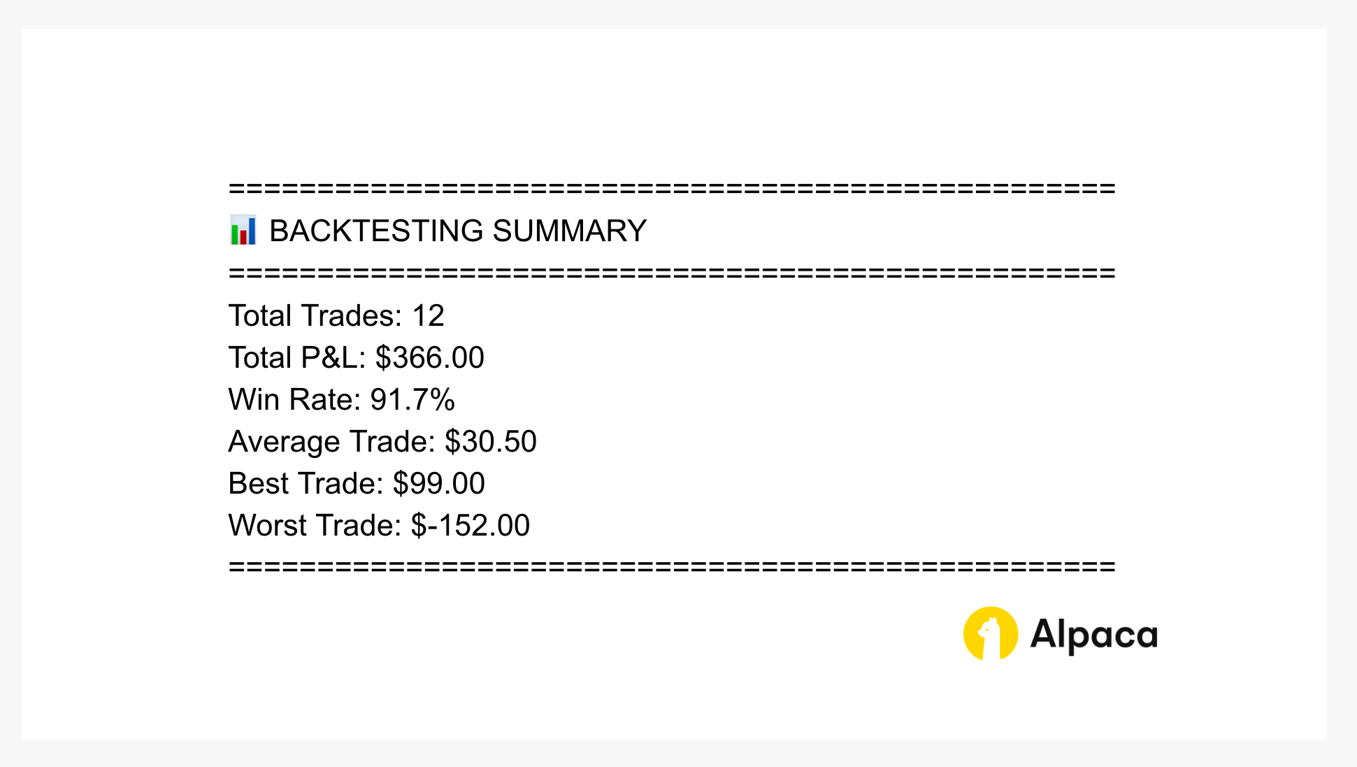
Performance Summary (As of July 21–25, 2025)

Over the backtesting period, the cumulative P&L finished at approximately $366.00 across 12 trades, with a win rate of about 91.7%. The average trade returned $30.50, with the best trade earning $99.00 and the worst losing $152.00.

The equity curve highlights a few drawdowns but an overall upward trajectory by the end of the test period. Please note these results are hypothetical and based on the assumptions described earlier. All investments involve risk, and the past performance of a security, or financial product does not guarantee future results or returns. There is no guarantee that any investment strategy will achieve its objectives.

Conclusion

Because options strategies can be complex and sensitive to volatility, time decay, and sudden price movements, thorough backtesting is especially important before trading live capital. Backtesting helps you explore how a strategy might have performed in different market conditions, understand potential risks, and refine your approach. These results are hypothetical and do not predict future performance, but they provide valuable context when evaluating a strategy.

Please note that this backtesting notebook uses signed Alpaca API clients with a custom user agent ('ZERO-DTE-NOTEBOOK') to help Alpaca identify usage patterns from educational backtesting notebooks and improve the overall user experience. You can opt out by replacing the `TradingClientSigned`, `OptionHistoricalDataClientSigned`, and `StockHistoricalDataClientSigned` classes with the standard `TradingClient`, `OptionHistoricalDataClient`, and `StockHistoricalDataClient` classes in the client initialization cell — though we kindly hope you'll keep it enabled to support ongoing improvements to Alpaca's educational resources.

We hope this guide helps you start backtesting and refining your own strategy. Share your results with our community and explore these resources:

• Sign up for an Alpaca Trading API account
• How to Trade Options with Alpaca’s Trading API
• Read more Options Trading Tutorials

If you want to know more about how to code alpaca-py, check out the following resources:

• Alpaca-py GitHub Page
• Alpaca-py Documentation
• API Reference of Alpaca APIs

---

*Limitations and key assumptions of backtesting experiment

• Liquidity (Assumed but Filtered)
  • While liquidity modeling is excluded, this backtest only uses option tick data with at least one transaction. This indirectly considers liquidity, as bid or ask prices would not be available otherwise. To achieve more realistic results, you can consider filtering potential contracts by size.
• Pricing of Bid-Ask Spreads: 
  • For option Greeks and implied volatility calculations, we use the midpoint of the bid-ask spreads. For all other order logic, we use the ask price for long put options and the bid price for short put options.
• Expects Early Assignment: 
  • We assume early assignment if the underlying price drops below 99.5% of the short strike, minus the premium received. The resulting loss is included in the backtest results. To disable or modify this assumption, adjust the logic in the trade_0DTE_options_historical function.
• Single-day Trading Only (0DTE): 
  • Orders must be placed at least one hour before expiration. Any orders submitted later will be considered invalid.
• Auto-Liquidation 
  • Before Expiration: All open positions are automatically closed starting 30 minutes before expiration for risk management purposes.

Options trading is not suitable for all investors due to its inherent high risk, which can potentially result in significant losses. Please read Characteristics and Risks of Standardized Options before investing in options.

Please note that we are using SPY as an example, and it should not be considered investment advice.

Alpaca and Databento are not affiliated and neither are responsible for the liabilities of the other. 

Past hypothetical backtest results do not guarantee future returns, and actual results may vary from the analysis.

Please note that this article is for general informational purposes only and is believed to be accurate as of the posting date but may be subject to change. The examples above are for illustrative purposes only.

All investments involve risk, and the past performance of a security, or financial product does not guarantee future results or returns. There is no guarantee that any investment strategy will achieve its objectives. Please note that diversification does not ensure a profit, or protect against loss. There is always the potential of losing money when you invest in securities, or other financial products. Investors should consider their investment objectives and risks carefully before investing.

The algorithm’s calculations are based on historical and real-time market data but may not account for all market factors, including sudden price moves, liquidity constraints, or execution delays. Model assumptions, such as volatility estimates and dividend treatments, can impact performance and accuracy. Trades generated by the algorithm are subject to brokerage execution processes, market liquidity, order priority, and timing delays. These factors may cause deviations from expected trade execution prices or times. Users are responsible for monitoring algorithmic activity and understanding the risks involved. Alpaca is not liable for any losses incurred through the use of this system.

The Paper Trading API is offered by AlpacaDB, Inc. and does not require real money or permit a user to transact in real securities in the market. Providing use of the Paper Trading API is not an offer or solicitation to buy or sell securities, securities derivative or futures products of any kind, or any type of trading or investment advice, recommendation or strategy, given or in any manner endorsed by AlpacaDB, Inc. or any AlpacaDB, Inc. affiliate and the information made available through the Paper Trading API is not an offer or solicitation of any kind in any jurisdiction where AlpacaDB, Inc. or any AlpacaDB, Inc. affiliate (collectively, “Alpaca”) is not authorized to do business.

Securities brokerage services are provided by Alpaca Securities LLC ("Alpaca Securities"), member FINRA/SIPC, a wholly-owned subsidiary of AlpacaDB, Inc. Technology and services are offered by AlpacaDB, Inc.

This is not an offer, solicitation of an offer, or advice to buy or sell securities or open a brokerage account in any jurisdiction where Alpaca Securities are not registered or licensed, as applicable.