In the first part of this series, we explored what 0DTE options are, discussing both the advantages and challenges of 0DTE strategies. We also explained how option Greeks like theta and delta impact them. In this guide, we’ll shift focus to the practical and technical side: building scripts and executing 0DTE strategies using Alpaca’s Trading API.
To get the most out of this guide, explore the following resources first:
Also, before diving into 0DTE options trading on Alpaca, keep these key points in mind:
- Important Notes:
- The code assumes a flat interest rate, excludes dividends, and is not optimized for 0DTE otpions. It does not consider market hours and serves as a starting point rather than a complete strategy.
- Expiration Day Order Rules:
- Orders must be submitted before 3:15 p.m. ET for stocks/options and 3:30 p.m. ET for broad-based ETFs (e.g., SPY, QQQ).
- Orders placed after these times will be rejected.
- Expiring positions are auto-liquidated at 3:30 p.m. ET (stocks/options) and 3:45 p.m. ET (broad-based ETFs) for risk management.
- American-Style Options Considerations:
- American-style options may be assigned early, affecting trade outcomes. Profit/loss scenarios assume expiration without early exercise and do not factor in transaction fees (e.g., brokerage fees, commissions). Traders should also monitor ex-dividend dates for short calls to manage assignment risk.
- Example equity:
- "SPY" is used for demonstration purposes and should not be considered investment advice.
Common 0DTE Strategies
While we went over these 0DTE strategies in more detail in our first 0DTE options blog, we thought it would be beneficial to provide a refresher on some of the more common ones:
Short Vertical Call Spread
A short vertical call spread is a credit spread constructed by selling a call option with a lower strike price (K1) and simultaneously buying a call option with a higher strike price (K2), both with the same expiration date. The net premium paid represents the maximum risk. The strategy profits if the underlying asset's price stays below K1 at expiration.
Short Vertical Put Spread
A short vertical put spread is a credit spread established by selling a put option with a higher strike price (K1) and simultaneously buying a put option with a lower strike price (K2), both with the same expiration date. The net premium received represents the maximum potential profit. This strategy is profitable if the underlying asset's price remains above K1 at expiration. The maximum loss is capped at the difference between the strike prices (K1 - K2) minus the initial credit received.
Iron Condor
An iron condor is a neutral, defined-risk strategy that profits from the underlying asset's price remaining within a predefined range at expiration. It consists of four options legs:
- Short OTM Call: Selling a call option with a strike price (K1) above the current underlying price.
- Long OTM Call: Buying a call option with a higher strike price (K2) than K1 to cap potential losses if the price rises significantly.
- Short OTM Put: Selling a put option with a strike price (K3) below the current underlying price.
- Long OTM Put: Buying a put option with a lower strike price (K4) than K3 to limit losses if the price falls significantly.
This structure creates two vertical spreads: a bearish call spread (K1 short, K2 long) and a bullish put spread (K3 short, K4 long). The maximum profit is achieved if the underlying price stays between K1 and K3 at expiration, allowing all short options to expire worthless. The maximum loss is capped at the difference between the wider spread's width and the net premium received.
Iron Butterfly
An iron butterfly is a neutral, defined-risk options strategy that profits from minimal movement in the underlying asset's price. It involves four options legs, all with the same expiration date, centered around a single, at-the-money (ATM) strike price (K):
- Short ATM Call: Selling a call option with strike price K.
- Short ATM Put: Selling a put option with strike price K.
- Long OTM Call: Buying a call option with a higher strike price (K1) to limit upside risk.
- Long OTM Put: Buying a put option with a lower strike price (K2) to limit downside risk.
The sold straddle (short ATM call and put) generates premium income, while the purchased OTM options cap potential losses. Maximum profit occurs if the underlying price remains at K at expiration, causing all options to expire worthless. Maximum loss is limited to the difference between the spread widths and the net premium received. Profit potential is typically higher than an iron condor, but so is the risk of loss if the underlying price moves significantly.
Risk-Reward Analysis in 0DTE Trading
In 0DTE trading, managing the balance between potential reward and risk is critical. One possible risk management approach is targeting a max loss to max profit ratio of approximately 3:1. This means that the potential loss on a trade should ideally not exceed three times the potential profit. This ratio aligns with the risk-reward structure of many defined-risk strategies, such as vertical spreads, where the maximum loss is capped but mostly higher than the premium collected.
A potential practice among traders is to sell vertical spreads to collect approximately one third of the width of the strike prices (the difference between the strike prices of the options you are selling and buying in the spread). For example, in a $5-wide spread, a trader would aim to collect a net premium of about $1.67. This approach balances potential reward (the collected premium) against potential risk (the remaining spread width minus the premium). By adhering to this guideline, traders can potentially structure trades that provide profit potential while limiting downside exposure.
The rapid time decay (theta) of 0DTE options increases the probability of the short options expiring worthless, benefiting the seller. However, the high delta and gamma sensitivity of 0DTE options can lead to rapid price fluctuations. Even small adverse price movements can erode profits or trigger stop-losses.
By focusing on these ratios and sticking to disciplined risk management practices, traders can better navigate the 0DTE trading.
Assessing Market Conditions
In 0DTE options trading, understanding several key factors, like the option Greeks, is essential for understanding market conditions.
For instance, high theta has the potential to benefit short-term strategies like 0DTE options. Theta measures the rate of time decay, and high theta indicates that the option’s premium decreases significantly as time passes. This helps option sellers potentially capture premiums quickly or buy back their positions at lower prices. In 0DTE trading, where expiration occurs within hours, this rapid decay can provide a distinct advantage for sellers in stable market conditions.
On the other hand, delta-driven setups may be suitable when a clear market direction is anticipated. Traders can use indicators, such as the advance/decline (A/D) line, to potentially gauge market direction before entering a trade. However, markets for 0DTE options, particularly on indices and ETFs, often lack clear directional trends. Delta in 0DTE trading is highly sensitive to even minor price movements because options nearing expiration can rapidly shift from OTM to in-the-money (ITM), and vice versa.
This heightened sensitivity to price changes is primarily due to gamma, which measures the rate of change of an option's delta. As an option approaches expiration, its gamma typically increases. This means that for 0DTE options, even a small change in the underlying asset's price can cause a significant shift in the option's delta.
For example, suppose the SPY moves up by $2. A 0DTE short put spread might experience a tenfold greater change in its delta compared to a similar 45DTE spread. This illustrates the increased directional risk associated with 0DTE options due to their high gamma.
Factoring in IV (vega) and current market trends can also help traders decide whether to focus on theta decay or directional price moves (delta). Implied volatility reflects the market’s expectations for future price volatility, and any increase in IV can have a substantial impact on option premiums.
When IV is high, it allows sellers to collect potentially larger premiums upfront, even on expiration day. However, higher IV also increases the risk of sharp, sudden price movements, which can lead to significant losses due to gamma risk and the lack of time for adjustments in 0DTE trades even if you implement multiple-leg strategies like vertical spreads.
Lastly, liquidity plays a key role in 0DTE trading by directly affecting the bid-ask spread, which impacts both entry and exit efficiency. 0DTE options, often in high demand, typically have narrower spreads, allowing traders to enter and exit trades more quickly and with lower slippage. This is especially important for 0DTE trades, where every minute counts. However, liquidity can vary depending on the underlying asset and market conditions.
Traders should prepare for all possible scenarios—whether the stock moves in their favor, against them, or remains stagnant. The unique dynamics of 0DTE options, such as rapid theta decay and heightened gamma sensitivity, require thorough preparation. That’s why backtesting options strategies and paper trading strategies is strongly encouraged to evaluate potential risks and rewards before live trading. This helps traders fine-tune their setups and avoid costly mistakes in this fast-paced environment.
Building a Vertical Spread Strategy with Alpaca's Trading API
In this guide, we’ll explore how to automate the implementation of a theoretical short put vertical spread for 0DTE options using Python, Alpaca’s Trading API, and our paper trading account. If you’re not connected, learn how to start paper trading with Alpaca.
By leveraging data-driven techniques, we’ll cover everything from filtering suitable option contracts and calculating critical metrics like delta and implied volatility, to how to execute trades and monitor them with predefined exit strategies. Whether you’re a seasoned options trader or just starting to explore automated trading, this walkthrough will provide you with a clear framework for trading 0DTE options efficiently and responsibly.
Step 1: Setting Up the Environment
The first step involves configuring the environment for trading a bear put spread and specifying your Alpaca Paper Trading API keys. This ensures your API connections and variable setup are secure and streamlined for data retrieval and trading operations.
Note: While we are using Jupyter Notebook for this tutorial, you can use Google Collab or any other IDE as your code environment. You can also find all of the below code on Alpaca’s Github page.
# Install the package `alpaca-py` to import it
!python3 -m pip install --upgrade alpaca-py

import pandas as pd
import numpy as np
from scipy.stats import norm
import alpaca
from scipy.optimize import brentq
from datetime import datetime, time
from zoneinfo import ZoneInfo

from alpaca.trading.client import TradingClient
from alpaca.trading.requests import (
    MarketOrderRequest,
    GetOptionContractsRequest,
    MarketOrderRequest,
    OptionLegRequest,
    ClosePositionRequest,
)
from alpaca.data.historical.option import OptionHistoricalDataClient
from alpaca.data.historical.stock import StockHistoricalDataClient, StockLatestTradeRequest
from alpaca.data.requests import OptionLatestQuoteRequest
from alpaca.trading.enums import (
    AssetStatus,
    ExerciseStyle,
    OrderSide,
    OrderClass,
    OrderType,
    TimeInForce,
    QueryOrderStatus,
    ContractType
)

# API credentials for Alpaca API
API_KEY = "YOUR_ALPACA_API_KEY_FOR_PAPER_TRADING"
API_SECRET = 'YOUR_ALPACA_API_SECRET_KEY_FOR_PAPER_TRADING'
BASE_URL = None
## We use paper enviornment for this example (Please do not modify this. This example is for paper trading only)
PAPER = True

# Initialize Alpaca clients
trade_client = TradingClient(api_key=API_KEY, secret_key=API_SECRET, paper=PAPER, url_override=BASE_URL)
option_historical_data_client = OptionHistoricalDataClient(api_key=API_KEY, secret_key=API_SECRET, url_override=BASE_URL)
stock_data_client = StockHistoricalDataClient(api_key=API_KEY, secret_key=API_SECRET)

# Below are the variables for developing this documents
# Please do not change these variables
trade_api_url = None
trade_api_wss = None
data_api_url = None
option_stream_data_wss = None

# Configuration
underlying_symbol = 'SPY'

# Set the timezone
timezone = ZoneInfo("America/New_York")

# Set expiration range for options
today = datetime.now().date()

# Define a 10% range around the underlying price
STRIKE_RANGE = 0.1

# Risk free rate for the options greeks and IV calculations
risk_free_rate = 0.01

# Set the open interest volume threshold
OI_THRESHOLD = 500

# Buying power percentage to use for the trade
BUY_POWER_LIMIT = 0.10

# Check account buying power
buying_power = float(trade_client.get_account().buying_power)

# Calculate the limit amount of buying power to use for the trade
buying_power_limit = buying_power * BUY_POWER_LIMIT

# Define delta thresholds
SHORT_PUT_DELTA_RANGE = (-0.42, -0.38)
LONG_PUT_DELTA_RANGE = (-0.22, -0.18)

# Set minimum credit percentage (33%)
MIN_CREDIT_PERCENTAGE = 0.33

# Set stop loss threshold as twice the initial total delta.
DELTA_STOP_LOSS_THRES = 2

# Set target profit and stop-loss levels
TARGET_STOP_LOSS_PERCENTAGE = 0.5
Initialize Alpaca Clients: Set up Alpaca trading and data clients. These are necessary for executing trades, fetching stock prices, and retrieving options data.
Define Key Variables: Set up constants like the underlying asset symbol (e.g., SPY), expiration date (today), strike price range (e.g., ±10% of the current price), and your buying power limit (e.g., 10% of your Alpaca’s total buying power). This helps streamline later functions for filtering options data.
Step 2: Fetching Market Data
With the environment configured, the next step is to collect real-time data for the underlying stock and its options.
# Get the latest price of the underlying stock
def get_underlying_price(symbol):

    # Get the latest trade for the underlying stock
    underlying_trade_request = StockLatestTradeRequest(symbol_or_symbols=symbol)
    underlying_trade_response = stock_data_client.get_stock_latest_trade(underlying_trade_request)
    return underlying_trade_response[symbol].price

# Get the latest price of the underlying stock
underlying_price = get_underlying_price(underlying_symbol)
print(f"{underlying_symbol} price: {underlying_price}")
Underlying Price: get_underlying_price function allows you to get the latest price of the underlying stock.
# Set the minimum and maximum strike prices based on the underlying price
min_strike = str(underlying_price * (1 - STRIKE_RANGE))
max_strike = str(underlying_price * (1 + STRIKE_RANGE))

# Function to check for 0DTE options
def get_0DTE_options(underlying_symbol):

    # Fetch the options data to add to the portfolio
    req = GetOptionContractsRequest(underlying_symbols=[underlying_symbol],
                                    strike_price_gte=min_strike,
                                    strike_price_lte=max_strike,
                                    status='active',
                                    expiration_date=today,
                                    root_symbol=underlying_symbol,
                                    type='put',
                                    )

    # Get option chain (zero_dte_option) of the underlying symbol
    zero_dte_options = trade_client.get_option_contracts(req).option_contracts

    return zero_dte_options
0DTE Option: With the get_0DTE_options function, we can extract the option chains that expire on the same day.
# Calculate implied volatility
def calculate_implied_volatility(option_price, S, K, T, r, option_type):

    # Define a reasonable range for sigma
    sigma_lower = 1e-6
    sigma_upper = 5.0  # Adjust upper limit if necessary

    # Check if the option is out-of-the-money and price is close to zero
    intrinsic_value = max(0, (S - K) if option_type == 'call' else (K - S))
    if option_price <= intrinsic_value + 1e-6:

        # print("Option price is close to intrinsic value; implied volatility is near zero.") # Uncomment for checking the status

        return 0.0

    # Define the function to find the root
    def option_price_diff(sigma):
        d1 = (np.log(S / K) + (r + 0.5 * sigma ** 2) * T) / (sigma * np.sqrt(T))
        d2 = d1 - sigma * np.sqrt(T)
        if option_type == 'call':
            price = S * norm.cdf(d1) - K * np.exp(-r * T) * norm.cdf(d2)
        elif option_type == 'put':
            price = K * np.exp(-r * T) * norm.cdf(-d2) - S * norm.cdf(-d1)
        return price - option_price

    try:
        return brentq(option_price_diff, sigma_lower, sigma_upper)
    except ValueError as e:
        print(f"Failed to find implied volatility: {e}")
        return None

# Calculate option Delta
def calculate_delta(option_price, strike_price, expiry, underlying_price, RISK_FREE_RATE, option_type):
    # Set the current date and time
    now = datetime.now(tz=timezone)
    # Calculate the time to expiry in years
    T = (expiry - now).total_seconds() / (365 * 24 * 60 * 60)
    # Set minimum T to avoid zero
    T = max(T, 1e-6)

    if T == 1e-6:
        print("Option has expired or is expiring now; setting delta based on intrinsic value.")
        if option_type == 'put':
            return -1.0 if underlying_price < strike_price else 0.0
        else:
            return 1.0 if underlying_price > strike_price else 0.0

    implied_volatility = calculate_implied_volatility(option_price, underlying_price, strike_price, T, RISK_FREE_RATE, option_type)
    if implied_volatility is None:
        print("Implied volatility could not be determined, skipping delta calculation.")
        return None

    d1 = (np.log(underlying_price / strike_price) + (RISK_FREE_RATE + 0.5 * implied_volatility ** 2) * T) / (implied_volatility * np.sqrt(T))
    delta = norm.cdf(d1) if option_type == 'call' else -norm.cdf(-d1)
    return delta
Calculate Implied Volatility (IV): IV is calculated using a custom function based on the Black-Scholes model. With the calculate_implied_volatility function, we can estimate IV for options, including edge cases (e.g., OTM options with low premiums). Here, we set reasonable sigmas between 1e-6 to 5.0 to calculate IV. Also, this function includes a minimum T safeguard system. To avoid division errors or invalid calculations when T approaches zero (e.g., for options expiring soon), a minimum value of 1e-6 is set for T.
Calculate Delta: Using the calculate_delta function to calculate delta, we measure the sensitivity of the option's price to changes in the underlying asset’s price. The calculate_delta function takes several inputs, including the option price, strike price, time to expiration (T), underlying asset price, risk-free rate, and the type of option (put or call). These inputs are processed through the Black-Scholes formula to calculate delta.
# Exit the spread by liquidating the position
def close_spread(short_symbol, long_symbol):

    # Close the long put by selling it
    trade_client.close_position(
        symbol_or_asset_id = long_symbol,
        close_options = ClosePositionRequest(qty = "1")
    )

    # Close the short put by buying it back
    trade_client.close_position(
        symbol_or_asset_id = short_symbol,
        close_options = ClosePositionRequest(qty = "1")
    )
Build Exit Strategy: Close_spread function is used to exit a trade (i.e. liquidate the position) by buying back the short put and selling the long put with ClosePositionRequest, triggered by either a delta stop-loss or a profit target condition, which we define in the following function trade_0DTE_options.
Step 3: Screening for Suitable Options, Placing the Trade, and Monitoring and Exiting the Trade
With metrics calculated, we proceed to identify the short and long puts for the vertical spread.
def find_short_and_long_puts(zero_dte_options, underlying_symbol, risk_free_rate, OI_THRESHOLD, short_put_delta_range, long_put_delta_range):
    """
    Identify the short put (delta ~ -0.40) and long put (delta ~ -0.20) from the options chain.
    Returns dictionaries containing details of the selected options.
    """
    underlying_price = get_underlying_price(underlying_symbol)
    short_put = None
    long_put = None

    for option_data in zero_dte_options:
        try:
            # Validate open interest and volume
            if option_data.open_interest is None or option_data.open_interest_date is None:
                continue
            if float(option_data.open_interest) <= OI_THRESHOLD:
                continue

            # Fetch the latest option quote
            option_symbol = option_data.symbol
            option_quote_request = OptionLatestQuoteRequest(symbol_or_symbols=option_symbol)
            option_quote = option_historical_data_client.get_option_latest_quote(option_quote_request)[option_symbol]
            print(f"Option symbol is: {option_symbol}")

            # Extract necessary data
            option_price = (option_quote.bid_price + option_quote.ask_price) / 2
            strike_price = float(option_data.strike_price)
            expiration_date_naive_dt = datetime.combine(option_data.expiration_date, time(16, 0)) # Set time to 4:00 PM
            expiry = expiration_date_naive_dt.replace(tzinfo=timezone)
            # expiry = pd.Timestamp(option_data.expiration_date).replace(hour=16, minute=0, second=0)

            # Calculate delta
            delta = calculate_delta(
                option_price=option_price,
                strike_price=strike_price,
                expiry=expiry,
                underlying_price=underlying_price,
                risk_free_rate=risk_free_rate,
                option_type='put'
            )
            print(f"Delta is: {delta}")

            # Create dictionaries for short and long puts based on delta thresholds
            if short_put_delta_range[0] <= delta <= short_put_delta_range[1]:
                short_put = {
                    'close_price': option_data.close_price,
                    'close_price_date': option_data.close_price_date,
                    'expiration_date': expiry,
                    'id': option_data.id,
                    'name': option_data.name,
                    'open_interest': option_data.open_interest,
                    'open_interest_date': option_data.open_interest_date,
                    'root_symbol': option_data.root_symbol,
                    'size': option_data.size,
                    'status': option_data.status,
                    'strike_price': strike_price,
                    'style': option_data.style,
                    'symbol': option_symbol,
                    'tradable': option_data.tradable,
                    'type': option_data.type,
                    'underlying_asset_id': option_data.underlying_asset_id,
                    'underlying_symbol': option_data.underlying_symbol,
                    'initial_delta': delta,
                    'initial_option_price': option_price,
                }
            elif long_put_delta_range[0] <= delta <= long_put_delta_range[1]:
                long_put = {
                    'close_price': option_data.close_price,
                    'close_price_date': option_data.close_price_date,
                    'expiration_date': expiry,
                    'id': option_data.id,
                    'name': option_data.name,
                    'open_interest': option_data.open_interest,
                    'open_interest_date': option_data.open_interest_date,
                    'root_symbol': option_data.root_symbol,
                    'size': option_data.size,
                    'status': option_data.status,
                    'strike_price': strike_price,
                    'style': option_data.style,
                    'symbol': option_symbol,
                    'tradable': option_data.tradable,
                    'type': option_data.type,
                    'underlying_asset_id': option_data.underlying_asset_id,
                    'underlying_symbol': option_data.underlying_symbol,
                    'initial_delta': delta,
                    'initial_option_price': option_price,
                }

            # Stop searching if both options are found
            if short_put and long_put:
                break

        except KeyError as e:
            print(f"Error processing option {option_symbol}: {e}")
            continue

    return short_put, long_put
Within the find_short_and_long_puts function, we use calculate_delta function to find the short put (delta ~ -0.40) and long put (delta ~ -0.20) from the options chain extracted by the get_0DTE_options function. We already define the delta thresholds as parameters outside the function, making them adjustable and easy to trace back.
The script below filters contracts based on the following criteria:
- Target Deltas: Filter for options with deltas close to -0.40 for the short put and -0.20 for the long put defined as
SHORT_PUT_DELTA_RANGEandLONG_PUT_DELTA_RANGE. - Spread Width: Ensure the spread width is within a defined range (e.g., $2–$5) to manage risk and maintain a reasonable risk-reward ratio.
- Credit Received: Check if the premium collected is at least one-third of the spread width, following standard risk-reward guidelines, adjusted by
MIN_CREDIT_PERCENTAGE.
def trade_0DTE_options(underlying_symbol, risk_free_rate, OI_THRESHOLD, short_put_delta_range, long_put_delta_range, min_credit_percentage, delta_stop_loss_thres, target_stop_loss_percentage):
    """
    Execute a 0DTE bull put vertical spread.
    """
    # Fetch zero DTE options
    zero_dte_options = get_0DTE_options(underlying_symbol)

    if not zero_dte_options:
        print("No 0DTE options available for the underlying symbol.")
        return

    # Find the short and long put options using the helper function
    short_put, long_put = find_short_and_long_puts(zero_dte_options, underlying_symbol, risk_free_rate, OI_THRESHOLD, short_put_delta_range, long_put_delta_range)

    if not short_put or not long_put:
        print("Could not find suitable options with 40 and 20 deltas.")
        return

    # Calculate the width of the spread
    spread_width = abs(short_put['strike_price'] - long_put['strike_price'])

    if not (2 <= spread_width <= 5):
        print(f"Spread width of {spread_width} is outside the target range of $2-$5; skipping this pair.")
        return

    # Calculate premium collected and check against threshold
    credit_received = short_put['initial_option_price'] - long_put['initial_option_price']
    min_credit_threshold = spread_width * min_credit_percentage

    if credit_received <= min_credit_threshold:
        print(f"Credit received {credit_received} is below minimum threshold {min_credit_threshold}; skipping trade.")
        return

    # Calculate profit/loss metrics
    max_profit = credit_received
    max_loss = spread_width * 100 - credit_received # Since we may have an obligation to buy 100 shares if assigned
    initial_total_delta = abs(short_put['initial_delta']) - abs(long_put['initial_delta'])
    delta_stop_loss = initial_total_delta * delta_stop_loss_thres # Default: 2 times of the initial delta when we enter the market

    print(f"Placing 0DTE Bull Put Spread on {underlying_symbol}:")
    print(f"Sell 40 Delta Put: {short_put['symbol']} (Strike: {short_put['strike_price']}, Premium: {short_put['initial_option_price']}, Delta: {short_put['initial_delta']})")
    print(f"Buy 20 Delta Put: {long_put['symbol']} (Strike: {long_put['strike_price']}, Premium: {long_put['initial_option_price']}, Delta: {long_put['initial_delta']})")
    print(f"Spread Width: {spread_width}, Credit received: {credit_received}, Max Profit: {max_profit}, Max Loss: {max_loss}")
    print(f"Initial Total Delta: {initial_total_delta}, Delta Stop-Loss Trigger: {delta_stop_loss}")

    # Create a list for the order request
    order_legs = []
    ## Append Long Put
    order_legs.append(OptionLegRequest(
        symbol=long_put["symbol"],
        side=OrderSide.BUY,
        ratio_qty=1
    ))
    ## Append Short Put
    order_legs.append(OptionLegRequest(
        symbol=short_put["symbol"],
        side=OrderSide.SELL,
        ratio_qty=1
    ))
    # Place the order for both legs simultaneously
    req = MarketOrderRequest(
        qty=1,
        order_class=OrderClass.MLEG,
        time_in_force=TimeInForce.DAY,
        legs=order_legs
    )
    trade_client.submit_order(req)
    print("Spread order placed successfully.")

    # Set target profit and stop-loss levels
    target_profit_price = credit_received * target_stop_loss_percentage  # Default: 50% of credit received

    # Monitor the spread for delta stop-loss and profit target
    while True:
        # Fetch the latest quote for each leg
        short_quote_req = OptionLatestQuoteRequest(symbol_or_symbols=[short_put['symbol']])
        long_quote_req = OptionLatestQuoteRequest(symbol_or_symbols=[long_put['symbol']])

        short_quote = option_historical_data_client.get_option_latest_quote(short_quote_req)[short_put['symbol']]
        long_quote = option_historical_data_client.get_option_latest_quote(long_quote_req)[long_put['symbol']]

        # Calculate the mid-price for each option as the current option price
        short_put_price = (short_quote.bid_price + short_quote.ask_price) / 2
        long_put_price = (long_quote.bid_price + long_quote.ask_price) / 2

        # Calculate the latest delta values for each option
        current_short_delta = calculate_delta(
            option_price=short_put_price,
            strike_price=short_put['strike_price'],
            expiry=short_put['expiration_date'],
            underlying_price=get_underlying_price(underlying_symbol),
            risk_free_rate=risk_free_rate,
            option_type='put'
        )

        expiration_date_naive_dt=datetime.combine(long_put['expiration_date'], time(16, 0)) # Set time to 4:00 PM

        current_long_delta = calculate_delta(
            option_price=long_put_price,
            strike_price=long_put['strike_price'],
            expiry=short_put['expiration_date'],
            underlying_price=get_underlying_price(underlying_symbol),
            risk_free_rate=risk_free_rate,
            option_type='put'
        )

        # Calculate current total delta and spread price
        current_total_delta = abs(current_short_delta) - abs(current_long_delta)
        current_spread_price = short_put_price - long_put_price

        # Exit for target profit
        if current_spread_price <= target_profit_price:
            close_spread(short_put['symbol'], long_put['symbol'])
            print(f"Exited spread for target profit at price {current_spread_price}")
            break

        # Check if the stop-loss condition based on delta is met
        if current_total_delta >= delta_stop_loss:
            close_spread(short_put['symbol'], long_put['symbol'])
            print(f"Exited spread for delta stop-loss at total delta {current_total_delta}")
            break

        time.sleep(180)  # Check every 3 minutes
Once the contracts are selected, the script places the trade by simultaneously selling the short put and buying the long put. Using Alpaca’s submit_order function, we automate these processes. However, a live trading algorithm should include checks for buying power to ensure sufficient margin is available for both legs of the trade. Alpaca’s trading_client.get_account function allows you to access details about your brokerage account like how much buying power you have. Error handling should also account for scenarios where one leg is executed but the other fails due to insufficient funds or other issues.
Additionally, the current implementation assumes a fixed quantity (qty=1) for each trade. Position sizing should ideally be determined dynamically based on the trader’s risk tolerance, available margin, and the maximum potential loss of the spread. This ensures that trades align with the trader's overall portfolio risk management strategy.
Keep in mind that the function ensures that no trade is executed unless all predefined conditions are met, preventing unnecessary or suboptimal positions from being entered.
After entering the trade, the script continuously monitors its performance to exit based on predefined conditions. These include:
- Target Profit: Exit when the spread price decreases to 50% of the initial credit received, as specified by the
target_profit_price. - Delta Stop-Loss: Exit if the total delta of the spread doubles, signaling increased risk. This is defined as
current_total_delta >= delta_stop_loss, wheredelta_stop_lossis set at twice the initial total delta.
The monitoring process only begins once the vertical spread has been successfully executed, ensuring resources are not wasted on nonexistent trades. This function also includes a built-in print system to provide real-time feedback, offering transparency and peace of mind during execution. For detailed debugging, optional print statements, such as #print(f"Skipping option {option_name} due to missing trade or quote data."), can be uncommented to enhance visibility during testing.
Step 4: Running the Trading Script with Error Handling
# Main block to place and monitor a single 0DTE trade
if __name__ == '__main__':
    try:
        trade_0DTE_options(underlying_symbol, risk_free_rate, OI_THRESHOLD, SHORT_PUT_DELTA_RANGE, LONG_PUT_DELTA_RANGE, MIN_CREDIT_PERCENTAGE, DELTA_STOP_LOSS_THRES, TARGET_STOP_LOSS_PERCENTAGE) # Enter the trade once and monitor it until exit
    except Exception as e:
        print(f"Error: {e}")
The final section of the script is the entry point for executing and monitoring the 0DTE short put vertical spread strategy. The if __name__ == "__main__": block ensures that the trade_0DTE_options function is only executed when the script is run directly, not when it is imported as a module.
This block attempts to initiate the trade setup, placement, and monitoring process using the trade_0DTE_options function. If any errors occur during execution, such as API issues or unexpected data, the try-except block catches the exception and prints an error message.
Paper Trading Your 0DTE Strategy on Alpaca
Testing your strategies in a paper trading environment is a crucial step in developing and refining any trading strategy, especially for options trading due to their risks. You can do this using Alpaca’s Paper Trading environment. This allows you to test your 0DTE options hypothesis around different risks, strategies, and parameters, allowing you to build confidence in your strategy while not risking any money upfront. Remember, paper trading is not a guarantee of future results, but it's a valuable tool for evaluating the potential risks and rewards of your 0DTE strategy.
Theoretical Iron Condor Case Study
To solidify the understanding of 0DTE option strategies, let's consider a hypothetical scenario of iron condor in this section. Please note that the values used here are for illustrative purposes only and do not represent actual market conditions.
Scenario
Remember that in an iron condor there are four positions: selling a call option, buying a call option, selling a put option, and buying a put option.
Assumptions:
- Underlying Asset Price (S): $550.00
- Days to Expiration (DTE): 0 (Expiration Today)
- Spread Width: $5.00 for both put and call spreads.
So to set up the iron condor position, you could buy and sell following options at different strike prices:
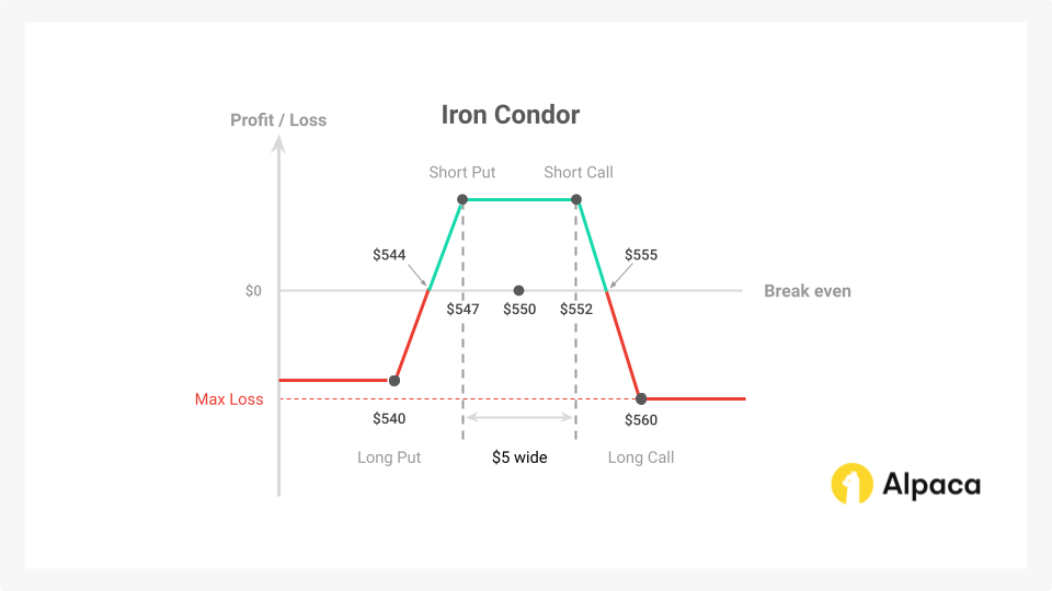
The total option premium collected in this scenario is $3.35 for shorting the $552 strike price put and the $547 strike price call. While the total premium paid is $0.35 for longing the $560 call and $540 put.
The net premium collected is then $3.00 since you will collect $3.35 for the short options and pay $0.35 for the long options. Note: We do not consider transaction fees (brokerage fees, commissions, etc.) here.
Maxim Profit
The maximum profit for this iron condor scenario is achieved if the underlying asset's price at expiration remains within the range defined by the short call strike ($552) and the short put strike ($547). In this scenario, all options expire out-of-the-money (OTM), and the iron condor's value becomes zero.
- Maximum Profit: $300.00
- Calculation: $3.00 (net premium collected) x 100 shares = $300.00 per Iron Condor
Maximum Loss
The maximum loss for this trade is $500.00. This is calculated by the $8.00 wide max spread width (call spread is a wider spread than that of put spread) minus the $3.00 net credit x 100 shares which equals $500.00 per iron condor sold.
Break Even
The lower breakeven price for this trade is $544.00 ($547.00 short put strike minus $3.00 iron condor credit equals $544.00). The $547.00 short put will have $3.00 of intrinsic value at expiration, while all of the other iron condor options will have expired worthless. Leaving you with a trade of $3.00, the same amount you sold the iron condor for at the time of entering the trade.
The upper breakeven price for this iron condor is $555.00 ($552.00 short call strike + $3.00 iron condor credit = $555.00). The $552.00 call option will have $3.00 of intrinsic value at expiration, while the put side will also expire worthless, exactly like with the lower breakeven.
Risk Reward Ratio
The risk-reward ratio refers to the ratio of the maximum potential loss to the maximum potential profit. Hence, it is $5.00 / $3.00 = 1.6667.
Strategy Summary
This guide explores 0DTE options trading using Alpaca’s Trading API, combining theoretical insights with practical execution to navigate 0DTE strategies.
Directional strategies, such as vertical call and put spreads, may be used by traders anticipating bearish or bullish market movements. Directionally neutral strategies, including iron condors, aim to profit from flat market conditions while managing risk under a certain level.
Key factors influencing 0DTE outcomes include using a possible risk-reward ratio approach where potential loss does not exceed three times the potential reward, and leveraging market dynamics. Rapid theta decay potentially benefits sellers by reducing option values near expiration, while high gamma increases sensitivity to price movements, raising directional risk. Implied volatility (IV) impacts premiums, typically offering higher earnings potential in high-IV environments but also increasing the risk of sudden price swings.
To connect theory with practice, we introduce a Python-based example to automate short put vertical spreads. This example demonstrates filtering options based on predefined deltas, setting up trades with a risk-reward balance, and managing positions using exit strategies like target profit and delta-based stop-loss triggers. This practical framework highlights how traders can execute and monitor 0DTE strategies efficiently with Alpaca’s Trading API.
Options trading is not suitable for all investors due to its inherent high risk, which can potentially result in significant losses. Please read Characteristics and Risks of Standardized Options before investing in options.
Past hypothetical backtest results do not guarantee future returns, and actual results may vary from the analysis.
The Paper Trading API is offered by AlpacaDB, Inc. and does not require real money or permit a user to transact in real securities in the market. Providing use of the Paper Trading API is not an offer or solicitation to buy or sell securities, securities derivative or futures products of any kind, or any type of trading or investment advice, recommendation or strategy, given or in any manner endorsed by AlpacaDB, Inc. or any AlpacaDB, Inc. affiliate and the information made available through the Paper Trading API is not an offer or solicitation of any kind in any jurisdiction where AlpacaDB, Inc. or any AlpacaDB, Inc. affiliate (collectively, “Alpaca”) is not authorized to do business.
Please note that this article is for general informational purposes only and is believed to be accurate as of the posting date but may be subject to change. The examples above are for illustrative purposes only.
All investments involve risk, and the past performance of a security, or financial product does not guarantee future results or returns. There is no guarantee that any investment strategy will achieve its objectives. Please note that diversification does not ensure a profit, or protect against loss. There is always the potential of losing money when you invest in securities, or other financial products. Investors should consider their investment objectives and risks carefully before investing.
Securities brokerage services are provided by Alpaca Securities LLC ("Alpaca Securities"), member FINRA/SIPC, a wholly-owned subsidiary of AlpacaDB, Inc. Technology and services are offered by AlpacaDB, Inc.
This is not an offer, solicitation of an offer, or advice to buy or sell securities or open a brokerage account in any jurisdiction where Alpaca Securities are not registered or licensed, as applicable.

