Understanding advanced options strategies can be challenging, especially when there are multiple contracts involved in a single trade, and this is the case with the iron condor. Whether you're looking to understand the theory or implement the strategy manually or algorithmically, this tutorial will explore the mechanics of iron condors, offering a clear breakdown of how the strategy operates and the risk-reward trade-offs it entails.

By combining theoretical foundations with actionable strategies for algorithmic integration, you'll gain a comprehensive understanding of iron condors and learn how to navigate their complexities for more informed decision-making in the options market.

What Is An Iron Condor?

The iron condor is a popular options trading strategy that is used to seek potential gain in neutral market conditions, though outcomes vary based on market conditions and execution. It consists of four options contracts at different strike prices, essentially the combination of a put spread and a call spread, forming a “condor” shape in the payoff diagram. Both spreads are made up of out-of-the-money (OTM) strike prices, allowing traders to potentially benefit from gradual change in price movement while limiting both potential gains and losses. 

An iron condor is considered a non-directional options strategy because it does not require price swings in specific direction, rather than accurately predicting which direction the market will lean towards. The strategies are often called the delta neutral strategy, which are influenced by the difference in option Greeks like low volatility (low vega) and time decay (theta). Please note when a trader wants to include at-the-money strike options in their position, an iron butterfly may be a suitable alternative to the iron condor. 

There are two primary variations of the iron condor: the short iron condor and the long iron condor.

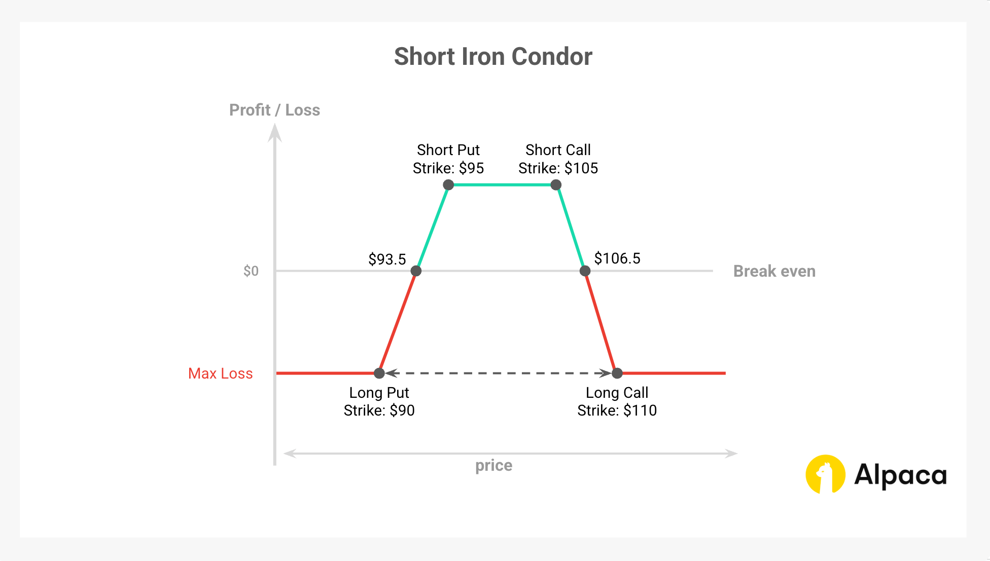
Short Iron Condor

A short iron condor is typically used by traders who anticipate a period of low volatility in the market. Rather than betting on price movement, this strategy potentially profits when the underlying asset stays within a narrow range. 

The Goal

The short iron condor aims to potentially capitalize on low volatility by collecting premiums from selling options, though it carries the risk of losses if the price moves beyond the breakeven points.

When To Use A Short Iron Condor

This strategy is often used when the following conditions are met:

• In relatively low volatility markets where price fluctuations are minimal.
• When assets are trading within a stable range (e.g., between $90 and $110) rather than those experiencing strong upward or downward trends.
• When implied volatility (IV) is high but expected to decrease over time.

Structure (Four Legs)

To create a short iron condor, a trader wants to build positions as:

1. Buy a lower put option (OTM)
2. Sell a middle put option (OTM)
3. Sell a middle call option (OTM)
4. Buy a higher call option (OTM)

Profit Potential

A short iron condor creates a range-bound profit zone between the short strikes. The potential for maximum profit is limited to the net premium received, while the theoretical maximum loss is defined and occurs if the price moves beyond the breakeven points.

• Theoretical maximum profit: The net premium received from the combination of the bull put spread and the bear call spread if they both expire worthless.
• Theoretical maximum loss: Often described as limited on each side; however, the risk can feel large if the underlying asset makes a big move. The theoretical maximum loss on either side is the difference between each vertical spread’s strike prices minus the total credit {(width of the wider spread – credit received) x 100}.

Example: Short Iron Condor (with payoff diagram)

To understand how an iron condor performs under various market conditions, let's analyze a short iron condor example using XYZ stock as the underlying asset. Since the profitability of an iron condor is mostly determined by the price range at expiration, it’s essential to consider these factors when constructing and managing the trade.

Example Setup:

• Underlying Price: XYZ is trading at $100.
• Initial Credit: ($1.50 (short call) + $1.50 (short put) - $0.75 (long call) - $0.75 (long put)) x 100 = $150.
• Theoretical maximum profit: $150 (same as the initial net credit)
• Theoretical maximum Loss: $350 (the difference between the width of the spread (whichever wider) ($5) minus the credit received ($1.50) × 100)
• Upper breakeven point: $106.50 (This value is determined by adding the initial credit received ($1.50) to the short call strike price ($105)).
• Lower breakeven point: $93.50 (This value is determined by subtracting the initial credit received ($1.50) from the short put strike price ($95)).

Scenario 1: XYZ is at $100 at expiration

• Both the short call ($105 strike) and short put ($95 strike) expire worthless.
• Since all options expire OTM, no further action is needed.
• Net Profit: $150 (initial credit) + $0 (all options expire) = $150 (theoretical maximum profit)

Scenario 2: XYZ is at $110 at expiration

• The short call ($105 strike) is in-the-money (ITM) and has an intrinsic value of $5.00 ($500 total).
• The long call ($110 strike) is OTM and expires worthless.
• The puts ($95 and $90 strikes) expire worthless.
• Net loss: $150 (initial credit) - $500 (loss on the short call position) = -$350 (theoretical maximum loss)

Scenario 3: XYZ is at $90 at expiration

• The short put ($95 strike) is ITM and has an intrinsic value of $5.00 ($500 total).
• The long put ($90 strike) is OTM and expires worthless.
• The calls ($105 and $110 strikes) expire worthless.
• Total loss: $150 (initial credit) - $500 (loss on the short put position) = -$350 (theoretical maximum loss)

Scenario 4: XYZ is at $106.5 or $93.5 at expiration (breakeven points)

• At $106.5, the short call is ITM by $1.5, leading to a $150 loss.
• At $93.5, the short put is ITM by $1.5, leading to a $150 loss.
• Breakeven: $150 (initial credit) - $150 (loss on either of the short options)  = $0

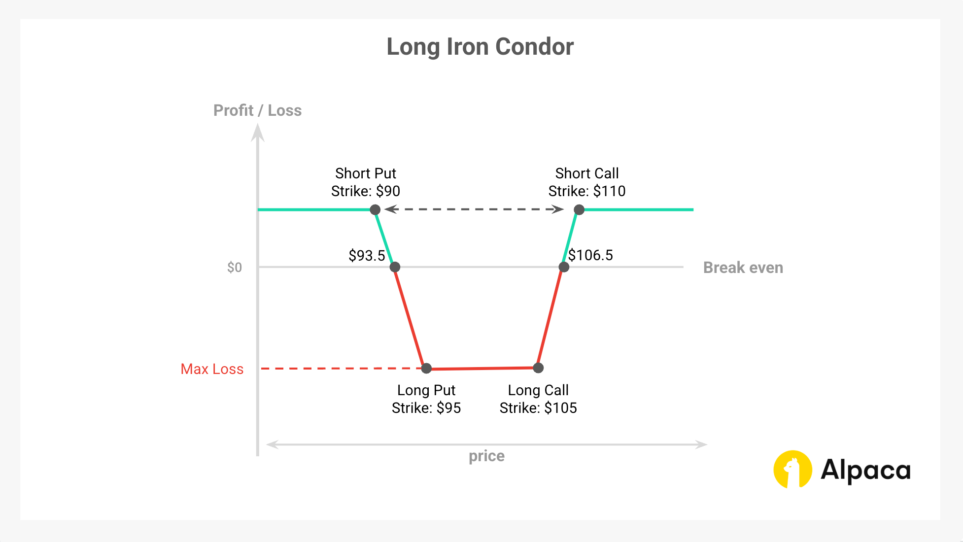
Long Iron Condor

The long iron condor is the opposite of the short version and may be used by traders who anticipate significant price movement. This strategy potentially benefits from volatility expansion and provides an opportunity for net profit if the underlying asset makes large moves in either direction.

The Goal

The long iron condor potentially profits from large price movements and increased volatility. Unlike the short iron condor, which relies on stability, the long version requires strong price swings beyond the middle strike prices.

When To Use An Iron Condor

This strategy is often used when the following conditions are met:

• High-volatility environments with expected price swings.
• When implied volatility is low but expected to rise.
• Before earnings announcements or major economic events.

Structure (Four Legs)

The long iron condor consists of following positions:

1. Sell a lower put option (OTM)
2. Buy a middle put option (OTM)
3. Buy a middle call option (OTM)
4. Sell a higher call option (OTM)

Profit Potential

The long iron condor has a loss zone between the short strikes and profits outside this range. This strategy has a limited downside but requires significant price movement to be profitable.

• Theoretical maximum profit: The difference between the strike prices of the bear put spread or the bull call spread, minus the net premium paid {(width of the wider spread−net debit paid) x 100}.
• Theoretical maximum loss: The net premium paid to establish the position.

Example: Long Iron Condor (with payoff diagram)

Let's go through the long iron condor example using XYZ stock as well. Since the profitability of an iron condor is mostly determined by the price range at expiration, it’s essential to consider these factors when constructing and managing the trade.

Example Setup:

• Underlying Price: XYZ is trading at $100.
• Net Debit: ($0.75 (short call) + $0.75 (short put) - $1.50 (long call) - $1.50 (long put)) x100 = -$150.
• Theoretical maximum profit: The difference between the width of the spread (whichever is wider) ($5) minus the debit paid ($1.50) × 100, which is $350 per contract.
• Theoretical maximum Loss: -$150 (same as the initial net debit)
• Upper breakeven point: $106.50 (This value is determined by adding the initial debit received ($1.50) to the long call strike price ($105)).
• Lower breakeven point: $93.50 (This value is determined by subtracting the initial debit received ($1.50) from the long put strike price ($95)).

Scenario 1: XYZ is at $100 at expiration

• All four legs expire worthless.
• The trader loses the full net debit of $150
• Since all options expire OTM, no further action is needed.
• Net loss: $0 (all options expire worthless) - $150 (initial debit) = -$150 (theoretical maximum loss)

Scenario 2: XYZ is at $110 at expiration

• The long call ($105 strike) is ITM and has an intrinsic value of $5.00 ($500 total).
• The short call ($110 strike) is ITM, but exercising the contract would be meaningless, as it would result in a net loss due to the premium and ultimately expire worthless.
• The puts ($95 and $90 strikes) expire worthless.
• Net profit: $500 (profit on the short call) - $150 (initial debit) = $350 (theoretical maximum profit)

Scenario 3: XYZ is at $85 at expiration

• The long put ($95 strike) is ITM and has an intrinsic value of $10.00 ($1,000 total).
• The short put ($90 strike) is ITM and most likely exercised (- $500 total)
• The calls ($105 and $110 strikes) expire worthless.
• Net profit: $1,000 (profit on the long put) - $500 (loss on the short put) - $150 (initial debit) = $350 (theoretical maximum profit)

Scenario 4: XYZ is at $106.5 or $93.5 at expiration (Breakeven Points)

• At $106.5, the short call is ITM by $1.5, leading to a $150 profit.
• At $93.5, the short put is ITM by $1.5, leading to a $150 profit.
• Breakeven: $150 (profit on either of the short options) - $150 (initial debit) = $0

Understanding The Greeks for An Iron Condor

Options traders use the Greeks to quantify risk and price behavior. Understanding how option Greeks impact an iron condor is crucial for effective risk management. Here, we cover the four main Greeks and discuss common benchmark values traders use for an iron condor.

Delta (Directional Exposure)

• Delta measures the sensitivity of the position to price changes.
• A well-structured iron condor should have a near-zero net delta at entry.
• As the underlying asset moves, delta changes, affecting potential adjustments.

Gamma (Rate of Change of Delta)

• Gamma is highest near expiration and impacts adjustments.
• A high gamma can cause rapid delta changes, increasing risk near expiration.
• A trader may aim to keep net vega between -0.05 and -0.15 for a short iron condor and between 0.05 and 0.15 for a long iron condor, ensuring the position can potentially benefit from changes in volatility.

Theta (Time Decay)

• Long option positions have negative theta, meaning they lose value over time.
• Short iron condors benefit from theta, as time decay erodes the value of sold options.
• Theta accelerates near expiration, favoring short strategies in stable markets.
• High volatility can offset theta gains, as price swings may exceed the expected range.
• A trader often targets a net theta, typically ranging from +0.05 to +0.15 per day for a short iron condor and -0.05 to -0.15 per day for a long iron condor.

Vega (Volatility Impact)

• Vega measures sensitivity to implied volatility changes.
• A short iron condor benefits from a decline in IV, while a long iron condor gains from an IV increase.
• Unexpected volatility spikes can drastically impact profitability.

Risk Management and Considerations

Proper risk management and position sizing may help optimize returns while limiting downside risk. Addressing these factors, traders may be able to quickly adjust their position based on market conditions, volatility. Below are some of the factors we considered when writing the iron condor.

Early Assignment Risk

• American-style options carry the risk of early assignment.
• Short ITM options in a short iron condor are at higher risk of assignment. If the underlying price moves beyond one of the short strikes, causing either the short call or short put to become in the money (ITM), the risk of early assignment increases. Conversely, this can be beneficial for a long iron condor.
• Strategies to mitigate early assignment: rolling positions, closing trades before expiration.

Volatility Risk

• A sudden increase in implied volatility (IV) can negatively impact a short iron condor while favoring a long iron condor.
• Monitoring IV trends and earnings events is crucial.
• Hedging strategies may involve adding a volatility hedge.

Time Decay and Its Double-Edged Sword

• Theta decay benefits short iron condors but can backfire if price swings are large.
• Close monitoring of price movements is essential.

Black Swan Events

• Market crashes or extreme price moves, while rare, can breach the defined risk boundaries and lead to significant losses.
• Tail risk hedging (e.g., deep OTM long options) can mitigate catastrophic losses.

Executing a Short Iron Condor Using Alpaca’s Trading API

This section provides a step-by-step guide to implementing a short iron condor using Python and Alpaca’s Trading API in the Paper Trading environment. The strategy is a four-legged, neutral strategy that involves simultaneously selling both an OTM call credit spread and an OTM put credit spread. This approach helps manage risk and optimize decision-making by leveraging key metrics and filters. If you’re not connected to Alpaca’s API or are unfamiliar with options trading, here are some useful resources to help you follow along:

• Sign up for an Alpaca Trading API account
• How to Connect to Alpaca's Trading API
• How to Start Paper Trading with Alpaca's Trading API
• How to Trade Options with Alpaca’s Trading API
• A Guide to Emotionless Options Trading

Important Notes:

• The code assumes a flat interest rate, excludes dividends, and is not optimized for 0DTE options. It does not consider market hours and serves as a starting point rather than a complete strategy.
• Expiration Day Order Rules:
  • Orders must be submitted before 3:15 p.m. ET for stocks/options and 3:30 p.m. ET for broad-based ETFs (e.g., SPY, QQQ).
  • Orders placed after these times will be rejected.
  • Expiring positions are auto-liquidated at 3:30 p.m. ET (stocks/options) and 3:45 p.m. ET (broad-based ETFs) for risk management.
• Multi-Leg (MLeg) Orders:
  • All legs of a strategy must be included in the same order for acceptance.
  • This is crucial for strategies with uncovered short options (e.g., short put calendar spreads, short call calendar spreads), which require Level 4 approval. See Alpaca's multi-leg order restrictions for details.
• American-Style Options Considerations:
  • American-style options may be assigned early, affecting trade outcomes. Profit/loss scenarios assume expiration without early exercise and do not factor in transaction fees (e.g., brokerage fees, commissions). Traders should also monitor ex-dividend dates for short calls to manage assignment risk.
• Example equity:
  • "JNJ" is used for demonstration purposes and should not be considered investment advice.

Setting Up the Environment and Trade Parameters

The first step involves configuring the environment for trading the short iron condor and specifying your Alpaca Paper Trading API keys. This ensures your API connections and variable setup are secure and streamlined for data retrieval and trading operations. 

Note: While we are using Jupyter Notebook for this tutorial, you can use Google Collab or any other IDE as your code environment. You can also find all of the below code on Alpaca’s Github page.

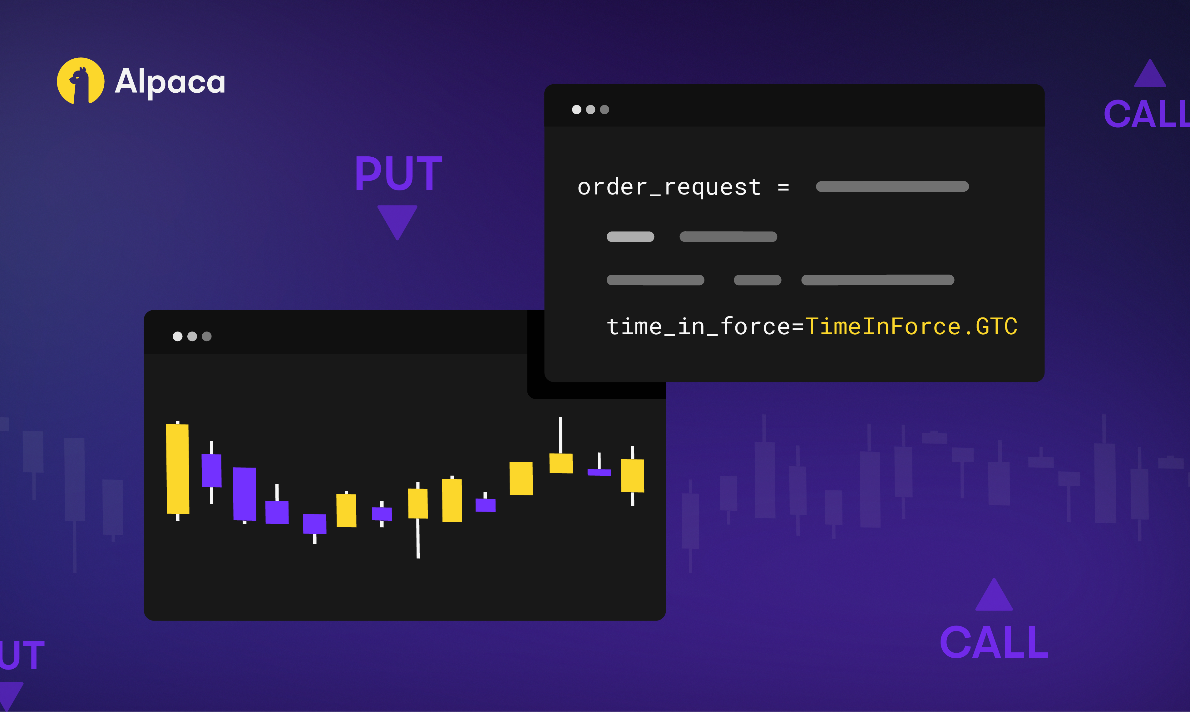
!pip install --upgrade alpaca-py
import pandas as pd
import numpy as np
from scipy.stats import norm
import alpaca
import time
from scipy.optimize import brentq
from datetime import datetime, timedelta
from zoneinfo import ZoneInfo
from alpaca.data.timeframe import TimeFrame, TimeFrameUnit
from dotenv import load_dotenv
import os

from alpaca.data.historical.option import OptionHistoricalDataClient
from alpaca.data.historical.stock import StockHistoricalDataClient, StockLatestTradeRequest
from alpaca.data.requests import StockBarsRequest, OptionLatestQuoteRequest, OptionChainRequest, OptionBarsRequest
from alpaca.trading.client import TradingClient
from alpaca.trading.requests import (
    MarketOrderRequest,
    GetOptionContractsRequest,
    MarketOrderRequest,
    OptionLegRequest,
    ClosePositionRequest,
)
from alpaca.trading.enums import (
    AssetStatus,
    ExerciseStyle,
    OrderSide,
    OrderClass,
    OrderStatus,
    OrderType,
    TimeInForce,
    QueryOrderStatus,
    ContractType,
)

The script initializes Alpaca clients for trading stocks and options, as well as for handling data requests.

# API credentials for Alpaca API
API_KEY = "YOUR_ALPACA_API_KEY_FOR_PAPER_TRADING"
API_SECRET = 'YOUR_ALPACA_API_SECRET_KEY_FOR_PAPER_TRADING'
BASE_URL = None
## We use a paper environment for this example (Please do not modify this. This example is for paper trading only)
PAPER = True

# Initialize Alpaca clients
trade_client = TradingClient(api_key=API_KEY, secret_key=API_SECRET, paper=PAPER, url_override=BASE_URL)
option_historical_data_client = OptionHistoricalDataClient(api_key=API_KEY, secret_key=API_SECRET, url_override=BASE_URL)
stock_data_client = StockHistoricalDataClient(api_key=API_KEY, secret_key=API_SECRET)

# Below are the variables for development this documents
# Please do not change these variables
trade_api_url = None
trade_api_wss = None
data_api_url = None
option_stream_data_wss = None

Calculations for Implied Volatility and Option Greeks with Black-Scholes model

The calculate_implied_volatility function estimates implied volatility (IV) using the Black-Scholes model. The function defines a reasonable range for sigma (1e-6 to 5.0) to avoid extreme values. For deep OTM options where the price is close to intrinsic value, the function directly sets IV to 0.0 to prevent calculation errors. A numerical root-finding method is used to solve for IV, ensuring accuracy even in edge cases.

# Calculate implied volatility
def calculate_implied_volatility(option_price, S, K, T, r, option_type):
    
    # Define a reasonable range for sigma
    sigma_lower = 1e-6
    sigma_upper = 5.0  # Adjust upper limit if necessary

    # Check if the option is out-of-the-money and price is close to zero
    intrinsic_value = max(0, (S - K) if option_type == 'call' else (K - S))
    if option_price <= intrinsic_value + 1e-6:
        
        print('Option price is close to intrinsic value; implied volatility is near zero.')
        return 0.0
    
    # Define the function to find the root
    def option_price_diff(sigma):
        d1 = (np.log(S / K) + (r + 0.5 * sigma ** 2) * T) / (sigma * np.sqrt(T))
        d2 = d1 - sigma * np.sqrt(T)
        if option_type == 'call':
            price = S * norm.cdf(d1) - K * np.exp(-r * T) * norm.cdf(d2)
        elif option_type == 'put':
            price = K * np.exp(-r * T) * norm.cdf(-d2) - S * norm.cdf(-d1)
        return price - option_price

    try:
        return brentq(option_price_diff, sigma_lower, sigma_upper)
    except ValueError as e:
        print(f"Failed to find implied volatility: {e}")
        return None

The calculate_greeks function estimates all option Greeks: delta, gamma, theta, and vega based on the implied volatility calculated through calculate_implied_volatility. In this demonstration, we mainly use delta and theta as well as implied volatility.

def calculate_greeks(option_price, strike_price, expiry, underlying_price, risk_free_rate, option_type):
    T = (expiry - pd.Timestamp.now()).days / 365 # It is unconventional, but some use 225 days (# of annual trading days) in replace of 365 days
    T = max(T, 1e-6)  # Set minimum T to avoid zero
    
    if T == 1e-6:
        print("Option has expired or is expiring now; setting Greeks based on intrinsic value.")
        if option_type == 'put':
            delta = -1.0 if underlying_price < strike_price else 0.0
        else:
            delta = 1.0 if underlying_price > strike_price else 0.0
        gamma = 0.0
        theta = 0.0
        vega = 0.0
        return delta, gamma, theta, vega
    
    # Calculate IV
    IV = calculate_implied_volatility(option_price, underlying_price, strike_price, T, risk_free_rate, option_type)
    print(f"implied volatility is {IV}")
    if IV is None or IV == 0.0:
        print("Implied volatility could not be determined, skipping Greek calculations.")
        return None
    
    d1 = (np.log(underlying_price / strike_price) + (risk_free_rate + 0.5 * IV ** 2) * T) / (IV * np.sqrt(T))
    d2 = d1 - IV * np.sqrt(T) # d2 for Theta calculation
    # Calculate Delta
    delta = norm.cdf(d1) if option_type == 'call' else -norm.cdf(-d1)
    # Calculate Gamma
    gamma = norm.pdf(d1) / (underlying_price * IV * np.sqrt(T))
    # Calculate Vega
    vega = underlying_price * np.sqrt(T) * norm.pdf(d1)
    # Calculate Theta
    if option_type == 'call':
        theta = (
            - (underlying_price * norm.pdf(d1) * IV) / (2 * np.sqrt(T))
            - (risk_free_rate * strike_price * np.exp(-risk_free_rate * T) * norm.cdf(d2))
        )
    else:
        theta = (
            - (underlying_price * norm.pdf(d1) * IV) / (2 * np.sqrt(T))
            + (risk_free_rate * strike_price * np.exp(-risk_free_rate * T) * norm.cdf(-d2))
        )
    # Convert annualized theta to daily theta
    theta /= 365
    
    return delta, gamma, theta, vega

Choosing the Right Strike Price and Expiration

Selecting the correct strike prices and expiration dates is important for optimizing a short iron condor. Since this strategy seeks to profit from range-bound market behavior, choosing strikes and expirations carefully can help balance risk and potential reward.

Strike Price Selection Using Option Moneyness:

• OTM Strikes: The short legs of the condor are often placed at OTM levels to collect premium while maintaining a reasonable probability of profit.
• ATM Strikes: These may offer higher premiums but increase directional risk if the underlying asset moves significantly. If you use the ATM option, it is regarded as an iron butterfly.
• ITM Strikes: Typically avoided due to increased capital requirements and reduced probability of success.

Expiration Timing:

• Short Leg Expiration: The short options are usually set to expire within 30-45 days to take advantage of time decay.
• Long Leg Expiration: The long options, acting as hedges, share the same expiration date as the short legs to avoid excessive complexity and assignment risk.
• Balancing Premium Collection and Risk: Selecting expirations with higher implied volatility can increase premium collection, but excessive IV exposure may introduce unwanted price swings.

By structuring the short iron condor with well-spaced OTM strikes and carefully chosen expiration dates, traders may better capture theta decay while attempting to mitigate the risk of large price movements.

Pick Your Strategy Inputs

Optimizing a short iron condor requires the use of historical data and statistical modeling to refine strike selection and expiration choice. 

The strategy can benefit from analyzing market conditions, including:

• Historical Volatility: Evaluating past price movements to determine an appropriate strike width and expiration period.
• Implied Volatility Skew: Identifying favorable IV levels to collect premium while being mindful of potential volatility spikes.
• Probability Models: Using statistical techniques to assess the likelihood of the underlying remaining within the defined range until expiration.
• Selecting the Right Underlying Stock:
  • Low Expected Price Movement: The strategy generally benefits from stocks with minimal expected volatility, increasing the chances that the price stays within the short strikes. Traders may consider avoiding stocks with a history of large post-earnings moves or high beta values. Stable large-cap stocks or ETFs such as SPY, QQQ, AAPL, and MSFT are commonly considered.
  • Sufficient Liquidity: High options trading volume (e.g., daily options volume > 200 contracts) and tight bid-ask spreads (e.g., $0.05 or less) may help improve execution efficiency and reduce slippage.
  • Stock Price Level Considerations: Stocks priced between $50 and $200 often offer a balance between strike spacing and premium collection without excessive risk.

By incorporating these factors, traders may enhance the performance of their short iron condor positions while working to manage exposure to unexpected volatility shifts.

Factor in Risk Management and Position Sizing

Risk management and position sizing are important components of maintaining the risk-reward balance when trading short iron condors. The strategy may adjust dynamically based on market conditions.

Adaptive Position Sizing:

• Capital Allocation: The strategy may limit trade allocation to a maximum of 5% of available capital to manage exposure.
• Strike Width Considerations: Wider spreads can increase potential profit but also elevate risk, requiring a balanced approach.
• Volatility-Based Adjustments: In times of high market volatility, strike widths may be adjusted to attempt to mitigate potential large price movements.

Stop-Loss Mechanisms:

• IV-Based Exit: You may set the system to trigger an early exit to help manage risk in case when implied volatility increases beyond expected levels.
• Profit Target Exit: Positions may be closed once a 30-50% profit threshold is reached to attempt to lock in gains before market conditions change.
• Delta Monitoring: The strategy may monitor delta exposure to help maintain a neutral stance and manage directional risk.
• Automated Cutoff Protection: Since early order cutoffs may affect liquidation timing, the algorithm seeks to manage positions before expiration risk escalates.

By implementing these risk management protocols, traders may better manage the stability and risk associated with short iron condor strategies while navigating changing market conditions.

# Select the underlying stock (Johnson & Johnson)
underlying_symbol = 'JNJ'

# Set the timezone
timezone = ZoneInfo('America/New_York')

# Get current date in US/Eastern timezone
today = datetime.now(timezone).date()

# Define a 15% range around the underlying price 
STRIKE_RANGE = 0.15

# Buying power percentage to use for the trade
BUY_POWER_LIMIT = 0.05

# Risk free rate for the options greeks and IV calculations
risk_free_rate = 0.01

# Check account buying power
buying_power = float(trade_client.get_account().buying_power)

# Set the open interest volume threshold
OI_THRESHOLD = 100

# Calculate the limit amount of buying power to use for the trade
buying_power_limit = buying_power * BUY_POWER_LIMIT

# Set the expiration date range for the options
min_expiration = today + timedelta(days=7)
max_expiration = today + timedelta(days=42)

# Get the latest price of the underlying stock
def get_underlying_price(symbol):
    # Get the latest trade for the underlying stock
    underlying_trade_request = StockLatestTradeRequest(symbol_or_symbols=symbol)
    underlying_trade_response = stock_data_client.get_stock_latest_trade(underlying_trade_request)
    return underlying_trade_response[symbol].price

# Get the latest price of the underlying stock
underlying_price = get_underlying_price(underlying_symbol)

# Set the minimum and maximum strike prices based on the underlying price
min_strike = str(underlying_price * (1 - STRIKE_RANGE))
max_strike = str(underlying_price * (1 + STRIKE_RANGE))

# Define a common expiration range for all legs between 14 days and 35 days
COMMON_EXPIRATION_RANGE = (14, 35)

# Each key corresponds to a leg and maps to a tuple of: (expiration range, IV range, delta range, theta range)
criteria = {
    'long_put':  (COMMON_EXPIRATION_RANGE, (0.15, 0.50), (-0.20, -0.01), (-0.1, -0.005)),
    'short_put': (COMMON_EXPIRATION_RANGE, (0.10, 0.40), (-0.30, -0.03), (-0.2, -0.01)),
    'short_call':(COMMON_EXPIRATION_RANGE, (0.10, 0.40), (0.03, 0.30), (-0.2, -0.01)),
    'long_call': (COMMON_EXPIRATION_RANGE, (0.15, 0.50), (0.01, 0.20), (-0.1, -0.005))
}

# Set target profit levels
TARGET_PROFIT_PERCENTAGE = 0.4

# Display the values
print(f"Underlying Symbol: {underlying_symbol}")
print(f"{underlying_symbol} price: {underlying_price}")
print(f"Strike Range: {STRIKE_RANGE}")
print(f"Buying Power Limit Percentage: {BUY_POWER_LIMIT}")
print(f"Risk Free Rate: {risk_free_rate}")
print(f"Account Buying Power: {buying_power}")
print(f"Buying Power Limit: {buying_power_limit}")
print(f"Open Interest Threshold: {OI_THRESHOLD}")
print(f"Minimum Expiration Date: {min_expiration}")
print(f"Maximum Expiration Date: {max_expiration}")
print(f"Minimum Strike Price: {min_strike}")
print(f"Maximum Strike Price: {max_strike}")

Factors To Include In Your Strategy

When implementing a short iron condor, it's essential to identify market conditions that support this strategy. Using a combination of price trends, volatility measures, and technical indicators, traders would be able to optimize entry points and improve trade efficiency. The following factors may help trigger the iron condor setups based on underlying asset price movement and volatility events.

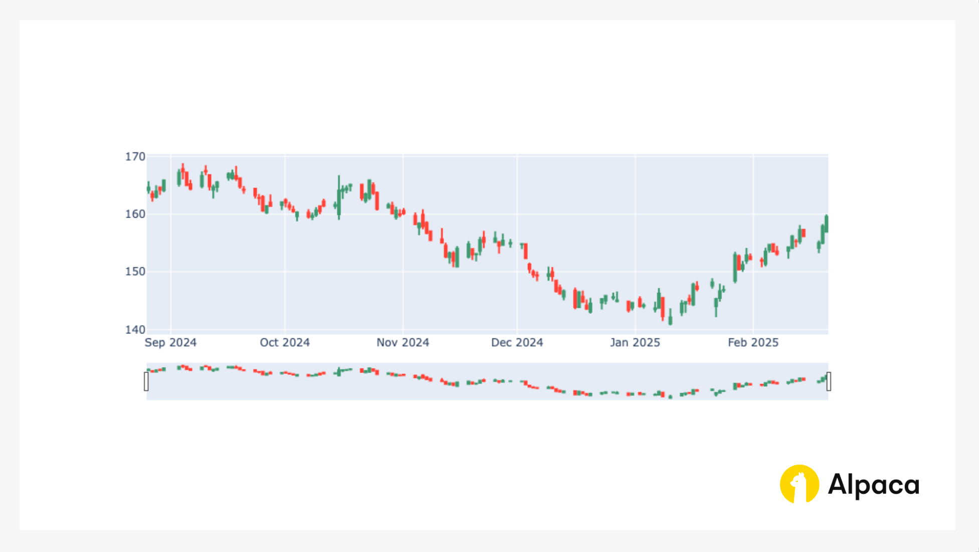
Stock Price Trends (Bar Chart Analysis)

Monitoring historical price movements helps traders assess the broader trend of the underlying asset. A candlestick chart provides insights into recent price action, as well as support and resistance levels, which can help determine whether the market is range-bound or trending. The iron condor strategy works better in elevated-volatility environments where volatility is expected to decrease, keeping the underlying asset stable within a defined range

# Get the historical data for the underlying stock by symbol and timeframe
# ref. https://alpaca.markets/sdks/python/api_reference/data/option/historical.html
def get_stock_data(underlying_symbol, days=90):
    today = datetime.now(timezone).date()
    req = StockBarsRequest(
        symbol_or_symbols=[underlying_symbol],
        timeframe=TimeFrame(amount=1, unit=TimeFrameUnit.Day),     # specify timeframe
        start=today - timedelta(days=days),                          # specify start datetime, default=the beginning of the current day.
    )
    return stock_data_client.get_stock_bars(req).df

priceData = get_stock_data(underlying_symbol, days=180)
# List of stock agg objects while dropping the symbol column
priceData = priceData.reset_index(level='symbol', drop=True)

import plotly.graph_objects as go

# Bar chart for the stock price
fig = go.Figure(data=[go.Candlestick(x=priceData.index,
                open=priceData['open'],
                high=priceData['high'],
                low=priceData['low'],
                close=priceData['close'])])

fig.show()

This code returns the bar chart like in the image below.

Relative Volatility Index (RVI)

The Relative Vigor Index (RVI) measures the strength of price momentum relative to volatility. It helps confirm whether the market is experiencing increased price fluctuations or stabilizing.

If the RVI is between 40 and 60, it suggests a moderately neutral volatility movement, which may be favorable as an entry point for a short iron condor strategy. Conversely, a low or declining RVI may indicate a stable market environment, making it a less favorable setup at the time of entry. However, since volatility contraction possibly benefits the strategy by accelerating premium decay in the sold options, it is important to actively monitor the RVI.

def calculate_rvi(df, period=14):
    # Calculate daily price changes 
    df["price_change"] = df["close"].diff()

    # Separate up and down price changes
    df['up_change'] = df['price_change'].where(df['price_change'] > 0, 0)
    df['down_change'] = -df['price_change'].where(df['price_change'] < 0, 0)

    # Calculate std of up and down changes over the rolling period
    df['avg_up_std'] = df['up_change'].rolling(window=period).std()
    df['avg_down_std'] = df['down_change'].rolling(window=period).std()

    # Calculate RVI
    df['rvi'] = 100 - (100 / (1 + (df['avg_up_std'] / df['avg_down_std'])))

    # Smooth the RVI with a 4 periods moving average
    df['rvi_smoothed'] = df['rvi'].rolling(window=4).mean()

    return df['rvi_smoothed']

# smoothed RVI
calculate_rvi(priceData, period=21).iloc[30:]

Bollinger Bands for Volatility Assessment

Bollinger Bands provide a dynamic range around the asset's price, helping to gauge market volatility. When the underlying stock price is near the upper Bollinger Band, it may indicate overbought conditions, while a price near the lower band suggests oversold levels. 

Short iron condor potentially benefits from moderate volatility when its expiry is close, where prices stay near the middle of the band rather than trending towards extreme levels. If the asset is trading closer to the upper or lower Bollinger Band, adjustments may be needed to avoid an early breakout risk.

# setup bollinger band calculations
def check_bb(df, period=14, multiplier=2):
    bollinger_bands = []
    # Calculate the Simple Moving Average (SMA)
    df['SMA'] = df['close'].rolling(window=period).mean()
    # Calculate the rolling standard deviation
    df['StdDev'] = df['close'].rolling(window=period).std()
    # Calculate the Upper Bollinger Band (two standard deviation)
    df['Upper Band'] = df['SMA'] + (multiplier * df['StdDev'])
    # Calculate the Lower Bollinger Band (two standard deviation)
    df['Lower Band'] = df['SMA'] - (multiplier * df['StdDev'])
    # Get the most recent Upper Band value
    upper_bollinger_band = df['Upper Band'].iloc[-1]
    lower_bollinger_band = df['Lower Band'].iloc[-1]
    
    bollinger_bands = [upper_bollinger_band, lower_bollinger_band]
    return bollinger_bands

bollinger_bands = check_bb(priceData, 14, 2)

print(f"Latest Upper Bollinger Band is: {bollinger_bands[0]}. Latest Lower Bollinger Band is {bollinger_bands[1]}; while underlying stock '{underlying_symbol}' price is {underlying_price}.")

Set up for a Short Iron Condor (Find both put and call options)

Both get_call_options and get_put_options functions fetch active options for a given underlying symbol within the specified strike price and expiration range.

# Check for call options
def get_call_options(underlying_symbol, min_strike, max_strike, min_expiration, max_expiration):
    
    # Fetch the options data to add to the portfolio
    req = GetOptionContractsRequest(
        underlying_symbols=[underlying_symbol],
        status=AssetStatus.ACTIVE,
        type=ContractType.CALL,
        strike_price_gte=min_strike,
        strike_price_lte=max_strike,
        expiration_date_gte=min_expiration,
        expiration_date_lte=max_expiration,
    )
    
    # Get call option chain of the underlying symbol
    call_options = trade_client.get_option_contracts(req).option_contracts
    return call_options

# Check for put options
def get_put_options(underlying_symbol, min_strike, max_strike, min_expiration, max_expiration):
    
    # Fetch the options data to add to the portfolio
    req = GetOptionContractsRequest(
        underlying_symbols=[underlying_symbol],
        status=AssetStatus.ACTIVE,
        type=ContractType.PUT,
        strike_price_gte=min_strike,
        strike_price_lte=max_strike,
        expiration_date_gte=min_expiration,
        expiration_date_lte=max_expiration,        
    )
    
    # Get put option chain of the underlying symbol
    put_options = trade_client.get_option_contracts(req).option_contracts
    return put_options

The helper function validate_sufficient_OI verifies that an option's data includes the necessary fields and that its open interest exceeds a specified threshold. It is used at the start of the workflow to ensure that only eligible options are processed further.

def validate_sufficient_OI(option_data, OI_THRESHOLD):
    '''Ensure that the option has the required fields and sufficient open interest.'''
    if option_data.open_interest is None or option_data.open_interest_date is None:
        return False
    if float(option_data.open_interest) <= OI_THRESHOLD:
        return False
    return True

The helper function build_option_dict constructs an option dictionary from option data and its calculated metrics. It is used within both check_candidate_option_conditions and find_options_for_short_iron_condor to store details for both the short put spread and short call spread, ultimately forming a complete short iron condor.

def build_option_dict(option_data, underlying_price, risk_free_rate):
    '''
    Helper to build an option dictionary from option_data and calculated metrics.
    '''
    # Retrieve the latest quote
    option_quote_req = OptionLatestQuoteRequest(symbol_or_symbols=option_data.symbol)
    option_quote = option_historical_data_client.get_option_latest_quote(option_quote_req)[option_data.symbol]
    option_price = (option_quote.bid_price + option_quote.ask_price) / 2

    strike_price = float(option_data.strike_price)
    expiration = pd.Timestamp(option_data.expiration_date)
    remaining_days = (expiration - pd.Timestamp.now()).days

    iv = calculate_implied_volatility(
        option_price=option_price,
        S=underlying_price,
        K=strike_price,
        T=max(remaining_days / 365, 1e-6),
        r=risk_free_rate,
        option_type=option_data.type.value
    )
    delta, _, theta, _ = calculate_greeks(
        option_price=option_price,
        strike_price=strike_price,
        expiration=expiration,
        underlying_price=underlying_price,
        risk_free_rate=risk_free_rate,
        option_type=option_data.type.value
    )

    # Build a candidate dictionary that can be augmented or returned
    candidate = {
        'id': option_data.id,
        'name': option_data.name,
        'symbol': option_data.symbol,
        'strike_price': option_data.strike_price,
        'root_symbol': option_data.root_symbol,
        'underlying_symbol': option_data.underlying_symbol,
        'underlying_asset_id': option_data.underlying_asset_id,
        'close_price': option_data.close_price,
        'close_price_date': option_data.close_price_date,
        'expiration': expiration,
        'remaining_days': remaining_days,
        'open_interest': option_data.open_interest,
        'open_interest_date': option_data.open_interest_date,
        'size': option_data.size,
        'status': option_data.status,
        'style': option_data.style,
        'tradable': option_data.tradable,
        'type': option_data.type,
        'initial_IV': iv,
        'initial_delta': delta,
        'initial_theta': theta,
        'initial_option_price': option_price,

    }
    return candidate

The helper function check_candidate_option_conditions checks if a candidate option meets the filtering criteria provided as a tuple (expiration range, IV range, delta range, theta range). It is used within the main workflow to determine whether a candidate qualifies for a specific leg of the iron condor.

def check_candidate_option_conditions(candidate, criteria, label):
    '''
    Check whether a candidate option meets the filtering criteria.
    The criteria is a tuple of (expiration_range, iv_range, delta_range, theta_range).
    '''
    expiration_range, iv_range, delta_range, theta_range = criteria

    if not (expiration_range[0] <= candidate['remaining_days'] <= expiration_range[1]):
        print(f"{candidate['symbol']} fails expiration condition for {label}.")
        return False
    if not (iv_range[0] <= candidate['initial_IV'] <= iv_range[1]):
        print(f"{candidate['symbol']} fails IV condition for {label}.")
        return False
    if not (delta_range[0] <= candidate['initial_delta'] <= delta_range[1]):
        print(f"{candidate['symbol']} fails delta condition for {label}.")
        return False
    if not (theta_range[0] <= candidate['initial_theta'] <= theta_range[1]):
        print(f"{candidate['symbol']} fails theta condition for {label}.")
        return False

    return True

The helper function pair_put_candidates identifies valid short and long put pairs for a bull put spread, ensuring the long put strike is below the short put strike and both are below the underlying price. This is essential for forming the put side of a short iron condor.

Similarly, pair_call_candidates selects short and long call pairs for a bear call spread, ensuring the short call strike is above the underlying price and below the long call strike. This function is key to assembling the call side of the iron condor.

def pair_put_candidates(short_puts, long_puts, underlying_price):
    '''
    For the bull put spread, we require: long_put strike < short_put strike < underlying_price
    '''
    for short_put in short_puts:
        for long_put in long_puts:
            if long_put['strike_price'] < short_put['strike_price'] and short_put['strike_price'] < underlying_price and long_put['strike_price'] < underlying_price:
                print(f"Selected put spread: short_put {short_put['symbol']} and long_put {long_put['symbol']}.")
                return short_put, long_put
    return None, None


def pair_call_candidates(short_calls, long_calls, underlying_price):
    '''
    For the bear call spread, we require: underlying_price < short_call strike < long_call strike
    '''
    for short_call in short_calls:
        for long_call in long_calls:
            if short_call['strike_price'] < long_call['strike_price'] and short_call['strike_price'] > underlying_price and long_call['strike_price'] > underlying_price:
                print(f"Selected call spread: short_call {short_call['symbol']} and long_call {long_call['symbol']}.")
                return short_call, long_call
    return None, None

The main function find_options_for_short_iron_condor orchestrates the entire process of constructing a short iron condor. It validates option data, builds full candidate dictionaries using build_option_dict, filters candidates with check_candidate_option_conditions, enforces a common expiration, pairs candidates via pair_put_candidates and pair_call_candidates, and finally checks risk parameters before returning the four legs of the iron condor.

def find_options_for_short_iron_condor(call_options, put_options, underlying_price, risk_free_rate, buying_power_limit, criteria, OI_THRESHOLD):
    '''
    Modular workflow to find an iron condor with a single common expiration.
    Returns a list of legs in the order:
       [short_put, long_put, short_call, long_call]
    '''
    common_expiration = None

    # Instead of immediately enforcing common expiration, store candidates by expiration date
    put_candidates_by_expiration = {}
    call_candidates_by_expiration = {}

    # Process put options
    for option_data in put_options:
        # If option does not meet the Open Interest Threshold, skip the process
        if not validate_sufficient_OI(option_data, OI_THRESHOLD):
            continue
        candidate = build_option_dict(option_data, underlying_price, risk_free_rate)
        
        # For puts, consider only options that are OTM (strike below underlying)
        if candidate['strike_price'] >= underlying_price:
            print(f"Skipping {candidate['symbol']}: not OTM for puts (strike {candidate['strike_price']} >= underlying {underlying_price}).")
            continue
        
        expiration = candidate['expiration']
        if expiration not in put_candidates_by_expiration:
            put_candidates_by_expiration[expiration] = {'long_put': [], 'short_put': []}
        
        # Add an option candidate to dictionary if it meets the criteria for 'long put'
        if check_candidate_option_conditions(candidate, criteria['long_put'], 'long_put'):
            put_candidates_by_expiration[expiration]['long_put'].append(candidate)
            print(f"Added {candidate['symbol']} as a long put candidate for expiration {expiration}.")

        # Add an option candidate to dictionary if it meets the criteria for 'short put'
        if check_candidate_option_conditions(candidate, criteria['short_put'], 'short_put'):
            put_candidates_by_expiration[expiration]['short_put'].append(candidate)
            print(f"Added {candidate['symbol']} as a short put candidate for expiration {expiration}.")

    # Process call options
    for option_data in call_options:
        if not validate_sufficient_OI(option_data, OI_THRESHOLD):
            continue
        candidate = build_option_dict(option_data, underlying_price, risk_free_rate)
        
        # For calls, consider only options that are OTM (strike above underlying)
        if candidate['strike_price'] <= underlying_price:
            print(f"Skipping {candidate['symbol']}: not OTM for calls (strike {candidate['strike_price']} <= underlying {underlying_price}).")
            continue
        
        expiration = candidate['expiration']
        if expiration not in call_candidates_by_expiration:
            call_candidates_by_expiration[expiration] = {'short_call': [], 'long_call': []}
        
        if check_candidate_option_conditions(candidate, criteria['short_call'], 'short_call'):
            call_candidates_by_expiration[expiration]['short_call'].append(candidate)
            print(f"Added {candidate['symbol']} as a short call candidate for expiration {expiration}.")
        if check_candidate_option_conditions(candidate, criteria['long_call'], 'long_call'):
            call_candidates_by_expiration[expiration]['long_call'].append(candidate)
            print(f"Added {candidate['symbol']} as a long call candidate for expiration {expiration}.")

    # Find common expiration(s) present in both puts and calls
    common_expirations = set(put_candidates_by_expiration.keys()).intersection(set(call_candidates_by_expiration.keys()))
    
    if not common_expirations:
        raise Exception('No common expiration found across put and call candidates.')

    # Choose the expiration with the most candidates
    selected_expiration = max(common_expirations, key=lambda exp: (len(put_candidates_by_expiration[exp]['long_put']) +
                                                        len(put_candidates_by_expiration[exp]['short_put']) +
                                                        len(call_candidates_by_expiration[exp]['short_call']) +
                                                        len(call_candidates_by_expiration[exp]['long_call'])))
    print(f"Selected common expiration: {selected_expiration}")

    # Use candidates only from the selected common expiration
    puts_for_selected_expiration = put_candidates_by_expiration[selected_expiration]
    calls_for_selected_expiration = call_candidates_by_expiration[selected_expiration]

    # Pair up the put candidates
    chosen_short_put, chosen_long_put = pair_put_candidates(puts_for_selected_expiration['short_put'], puts_for_selected_expiration['long_put'], underlying_price)
    # Pair up the call candidates
    chosen_short_call, chosen_long_call = pair_call_candidates(calls_for_selected_expiration['short_call'], calls_for_selected_expiration['long_call'], underlying_price)

    if not (chosen_short_put and chosen_long_put and chosen_short_call and chosen_long_call):
        raise Exception('Could not find a valid combination for the iron condor for the selected expiration.')

    # Check buying power requirements
    # For puts: maximum risk = (short_put strike - long_put strike) * option size
    # For calls: maximum risk = (long_call strike - short_call strike) * option size
    option_size = float(chosen_short_put['size'])
    risk_put = (chosen_short_put['strike_price'] - chosen_long_put['strike_price']) * option_size
    risk_call = (chosen_long_call['strike_price'] - chosen_short_call['strike_price']) * option_size

    print(f"Calculated bull put spread risk: {risk_put}, bear call spread risk: {risk_call}.")
    if risk_put >= buying_power_limit or risk_call >= buying_power_limit:
        raise Exception('Buying power limit exceeded for the iron condor risk.')

    # Return the four legs in the following order
    iron_condor = [chosen_short_put, chosen_long_put, chosen_short_call, chosen_long_call]
    print('\nReturning iron condor legs:')
    for leg in iron_condor:
        print(f"{leg['symbol']} at strike {leg['strike_price']}")
    return iron_condor

Execute your Short Iron Condor

You can run the find_options_for_short_iron_condor function to find a reasonable set of call options for a short iron condor.

call_options = get_call_options(underlying_symbol, min_strike, max_strike, min_expiration, max_expiration)
put_options = get_put_options(underlying_symbol, min_strike, max_strike, min_expiration, max_expiration)
iron_condor_order_legs = find_options_for_short_iron_condor(call_options, put_options, underlying_price, risk_free_rate, buying_power_limit, criteria, OI_THRESHOLD)

After running the code, you would see output similar to what is shown below, though it may vary depending on the specific conditions and stocks used.

Selected common expiration: 2025-03-21 00:00:00
Selected put spread: short_put JNJ250321P00145000 and long_put JNJ250321P00140000.
Selected call spread: short_call JNJ250321C00165000 and long_call JNJ250321C00175000.
Calculated bull put spread risk: 500.0, bear call spread risk: 1000.0.

Returning iron condor legs:
JNJ250321P00145000 at strike 145.0
JNJ250321P00140000 at strike 140.0
JNJ250321C00165000 at strike 165.0
JNJ250321C00175000 at strike 175.0

The script below builds the list of options for the short iron condor and places an order.

# iron_condor_order_legs = find_options_for_short_iron_condor(call_options, put_options, underlying_price, risk_free_rate, buying_power_limit, criteria, OI_THRESHOLD)

# # Place orders for the iron condor spread if all options are found
if iron_condor_order_legs:
    # Create a list for the order request
    order_legs = []
    ## Append short put
    order_legs.append(OptionLegRequest(
        symbol=iron_condor_order_legs[0]["symbol"],
        side=OrderSide.SELL,
        ratio_qty=1
    ))
    ## Append long put
    order_legs.append(OptionLegRequest(
        symbol=iron_condor_order_legs[1]["symbol"],
        side=OrderSide.BUY,
        ratio_qty=1
    ))
    ## Append short call
    order_legs.append(OptionLegRequest(
        symbol=iron_condor_order_legs[2]["symbol"],
        side=OrderSide.SELL,
        ratio_qty=1
    ))
    ## Append long call
    order_legs.append(OptionLegRequest(
        symbol=iron_condor_order_legs[3]["symbol"],
        side=OrderSide.BUY,
        ratio_qty=1
    ))

    # Place the order for both legs simultaneously
    req = MarketOrderRequest(
        qty=1,
        order_class=OrderClass.MLEG,
        time_in_force=TimeInForce.DAY,
        legs=order_legs
    )
    res = trade_client.submit_order(req)
    print("Short Iron Condor order placed successfully.")

Before the order is filled, traders may choose to cancel it. Please note that individual legs cannot be canceled or replaced. You must cancel the entire order. If you are not familiar with the level 3 option trading with multi-legs, please check out an example code for multi-leg option trading on Alpaca’s Github page!

# Query by the order's id
q1 = trade_client.get_order_by_client_id(res.client_order_id)

# Replace overall order
if q1.status != OrderStatus.FILLED:
    # Cancel the whole order
    trade_client.cancel_order_by_id(res.id)
    print(f"Canceled order: {res}")

else:
    print("Order is already filled.")

The Importance of Backtesting an Iron Condor Strategy

Backtesting your options strategy is a critical step in developing a robust iron condor strategy, especially when implementing it in an algorithmic trading system. Given that the short iron condor rely on volatility shifts (vega), and limited directional exposure (gamma), backtesting allows traders and quants to validate strategy performance before risking capital.

With Alpaca’s Trading API, you can not only backtest using an underlying asset’s historical data but also extract historical option data.

The script below retrieves historical option data. However, accessing the latest OPRA data may require the Algo Trader Plus subscription. Meanwhile, the free 'Basic' account typically provides the necessary historical data.

# Initialize the Option Historical Data Client
option_historical_data_client = OptionHistoricalDataClient(
    api_key=API_KEY, 
    secret_key=API_SECRET, 
    url_override=BASE_URL
)

# Define the request parameters
req = OptionBarsRequest(
    #  iron_condor_order_legs[1]["symbol"] = the short put option
    symbol_or_symbols=iron_condor_order_legs[1]["symbol"],
    timeframe=TimeFrame.Day,  # Choose timeframe (Minute, Hour, Day, etc.)
    start="2025-01-01",  # Start date
    end="2025-03-21"  # End date
)

option_historical_data_client.get_option_bars(req)

The partial output would look like below.
{   'data': {   'JNJ250321P00140000': [ {.....},
               {   'close': 0.14,
                   'high': 0.2,
                   'low': 0.12,
                   'open': 0.15,
                   'symbol': 'JNJ250321P00140000',
                   'timestamp': datetime.datetime(2025, 2, 19, 5, 0, tzinfo=TzInfo(UTC)),
                   'trade_count': 59.0,
                   'volume': 441.0,
                   'vwap': 0.157596},
               {   'close': 0.11,
                   'high': 0.12,
                   'low': 0.1,
                   'open': 0.1,
                   'symbol': 'JNJ250321P00140000',
                   'timestamp': datetime.datetime(2025, 2, 20, 5, 0, tzinfo=TzInfo(UTC)),
                   'trade_count': 15.0,
                   'volume': 71.0,
                   'vwap': 0.110704}
]
}

Trading an Iron Condor on Alpaca’s Dashboard

You can also execute an iron condor using Alpaca’s dashboard manually.

Please note we are using JNJ as an example and it should not be considered investment advice.

1. Log in to your account

Sign in to your account and navigate to the “Home” page.

2. Find your desired trade

On your dashboard in the top left, you can select between using your paper trading or live accounts. It’s important that you select the appropriate trading account before implementing an options strategy. If you want to practice without the risk of real capital, you can use your paper trading accounts. If you are looking to implement strategies, you can use your live account.

Once you’ve selected the desired account within your dashboard, you can monitor your portfolio, access market data, execute trades, and review your trading history. In order to create your first options trade, use the search bar to find and select the applicable option ticker symbol.

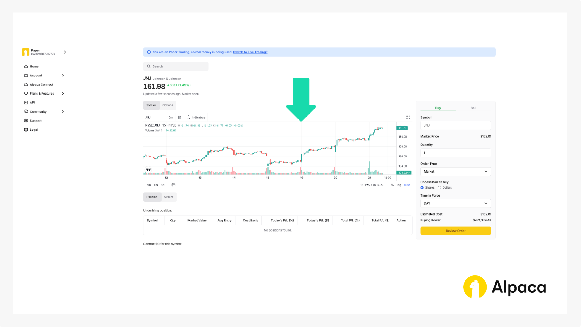
3. Check underlying security’s bar chart

If you search your desired underlying asset, a page shows the asset’s bar chart. You can use this bar chart for a simple analysis.

4. Opening an options position

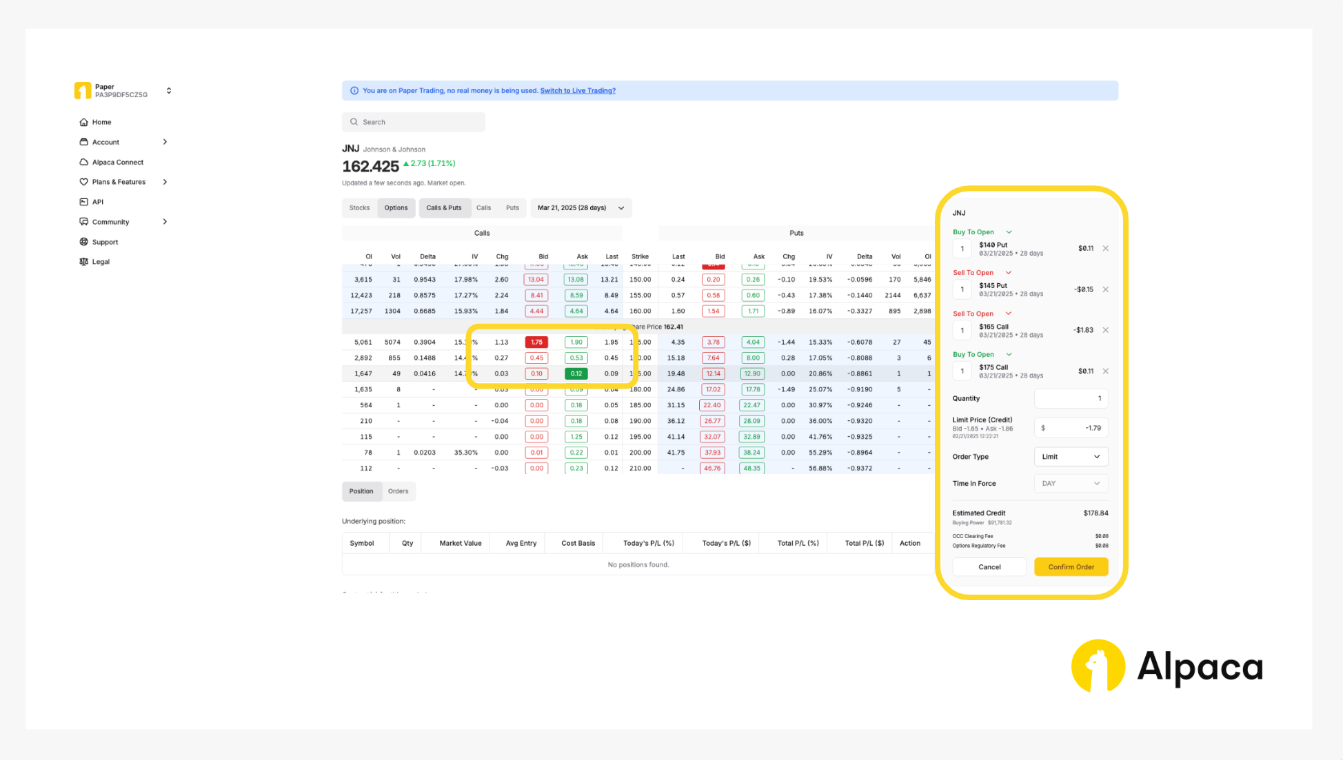
Assume we have already analyzed the market and determined the strike price for all four legs as follows: long put option to be $140.00; short put to be $145.00; short call to be $165.00; long call to be $175.00 at the expiration date of March 21, 2025. Once determined, select and review your order type (market or limit) and decide on the number of contracts you’d like to trade. You can select up to four legs. 

On the asset’s page, toggle from “Stocks” to “Options” and determine your desired contract type between calls and puts. You can also adjust the expiration date from the dropdown, ranging anywhere from 0DTE options to contracts hundreds of days in the future.

A short iron condor, for example, requires shorting OTM put and call options and longing further OTM put and call options at the same expiration date. Therefore, you can establish your position in the dashboard by selecting one short put option with “Sell To Open;” one short call option with “Sell To Open;” one long put option with “Buy To Open;” and one long call option with “Buy To Open” to purchase the options contracts.

Please note: The order in which you select the options does not matter. Additionally, on Alpaca’s dashboard and Trading API, credits are displayed as negative values, while debits appear as positive values. For example, in the image below, a credit spread (where your initial entry earns net profit) is shown with a negative limit price ($-1.79 in this case) under 'Limit Price (Credit),' reflecting a total credit of $178.84.

Once selected, review your order type (such as market, limit, stop, stop limit, or trailing stop) and the number of contracts you’d like to trade. Click the “Confirm Order” button on the bottom right.

Your paper trading account will then mimic the execution of the order as though it were a real transaction.

Optional: Cancel your order

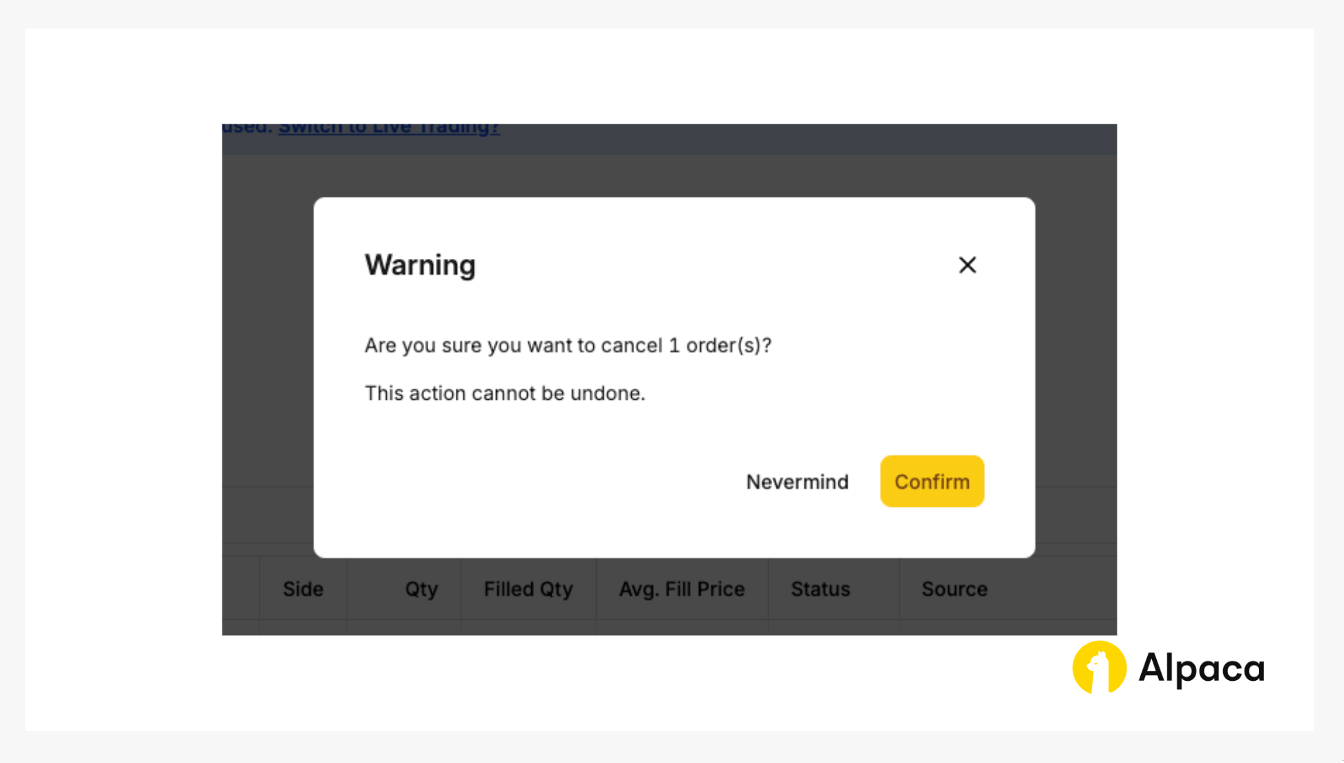
Keep in mind that with a multi-leg options order, you cannot cancel or replace an individual child leg. You can only cancel or replace the entire multi-leg options order. To do this, navigate to the 'Order' section, select the order you want to cancel, and click the 'Cancel 1 selected' button.

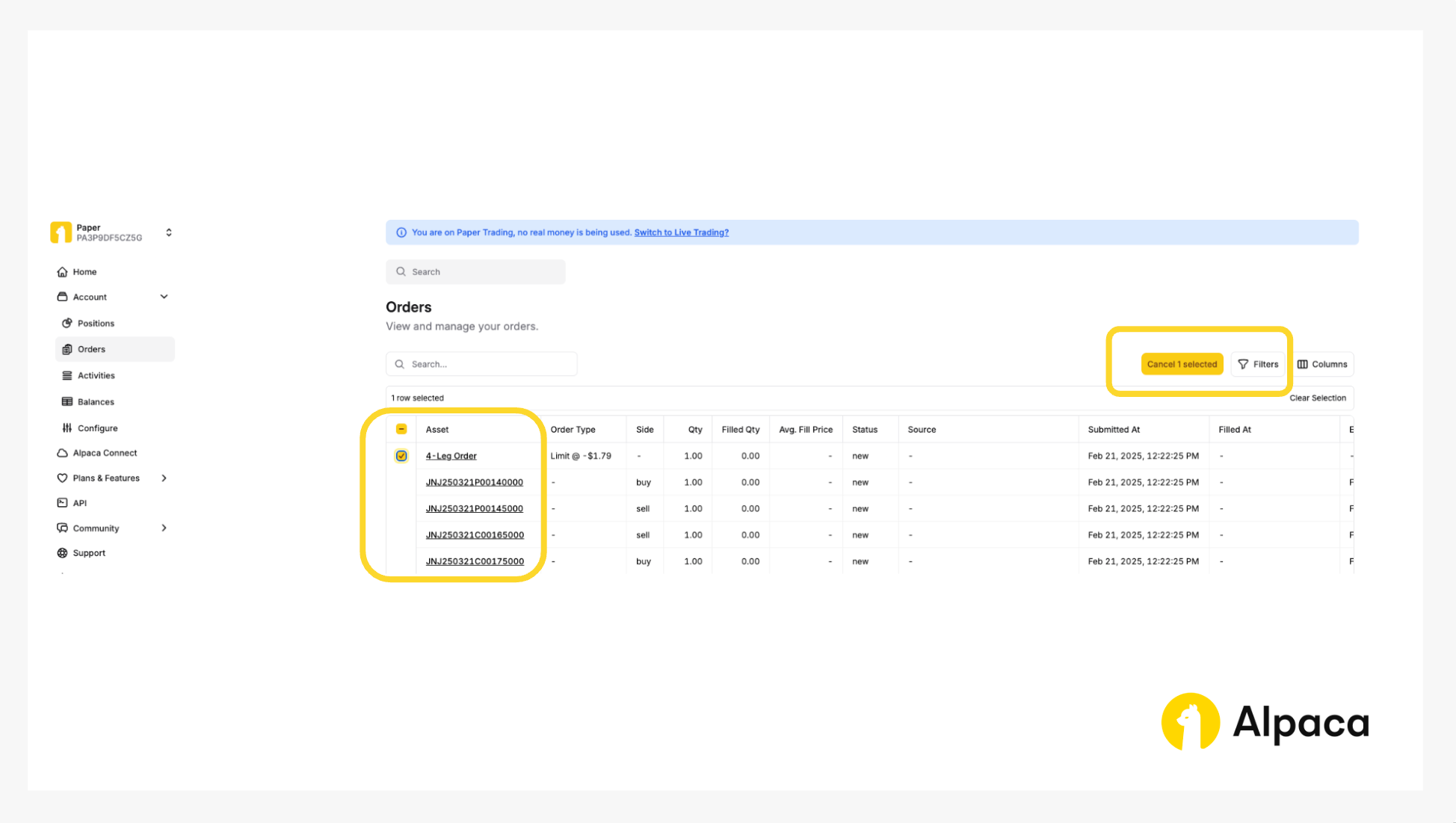
You’ll then be prompted to confirm.

5. Closing your position

Closing an options position involves selling the options contract that you previously bought (in a long position) or buying back the options contract that you previously sold (in a short position). Either action terminates, or “closes”, your associated position.

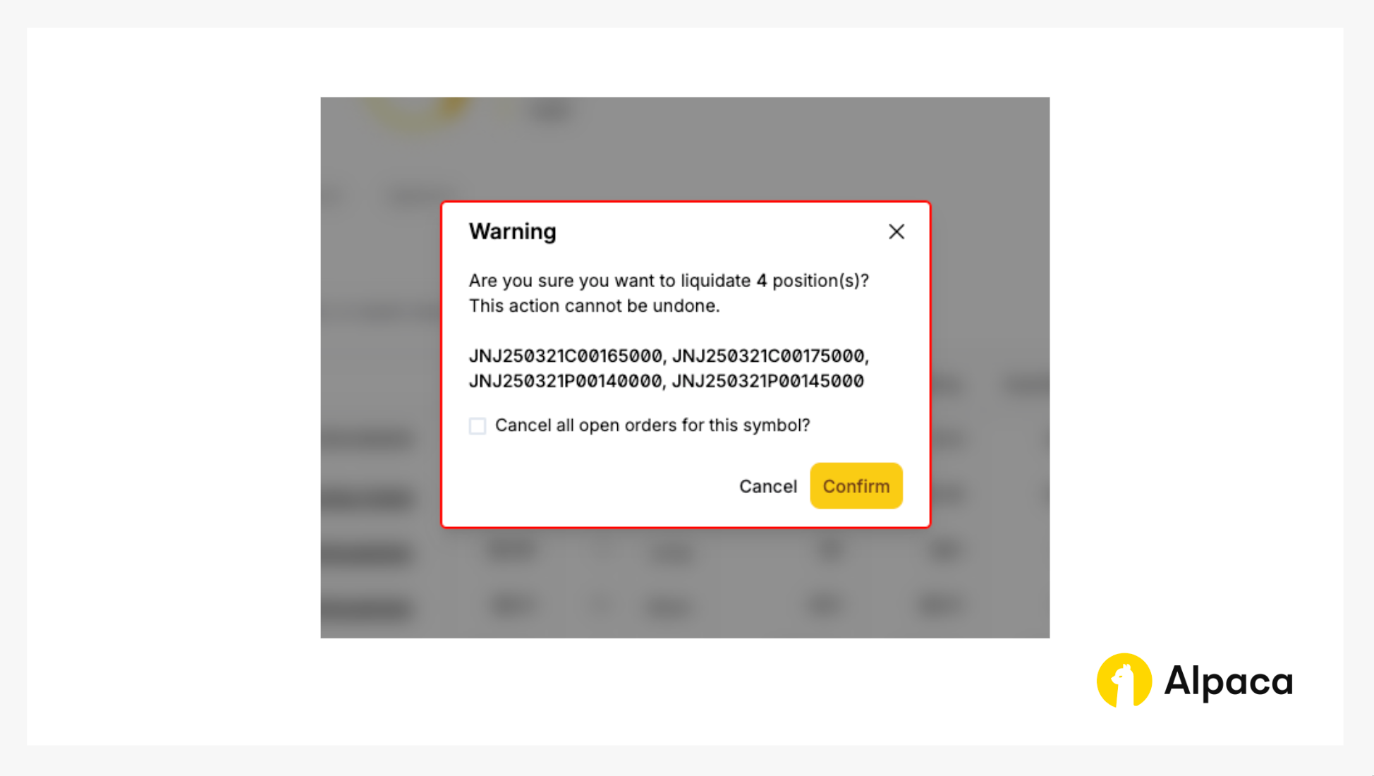
If you’d like to close your position, find the desired options contract on your “Home” page or under “Positions”. Click on the appropriate contract symbol and select “Liquidate 4 selected”.

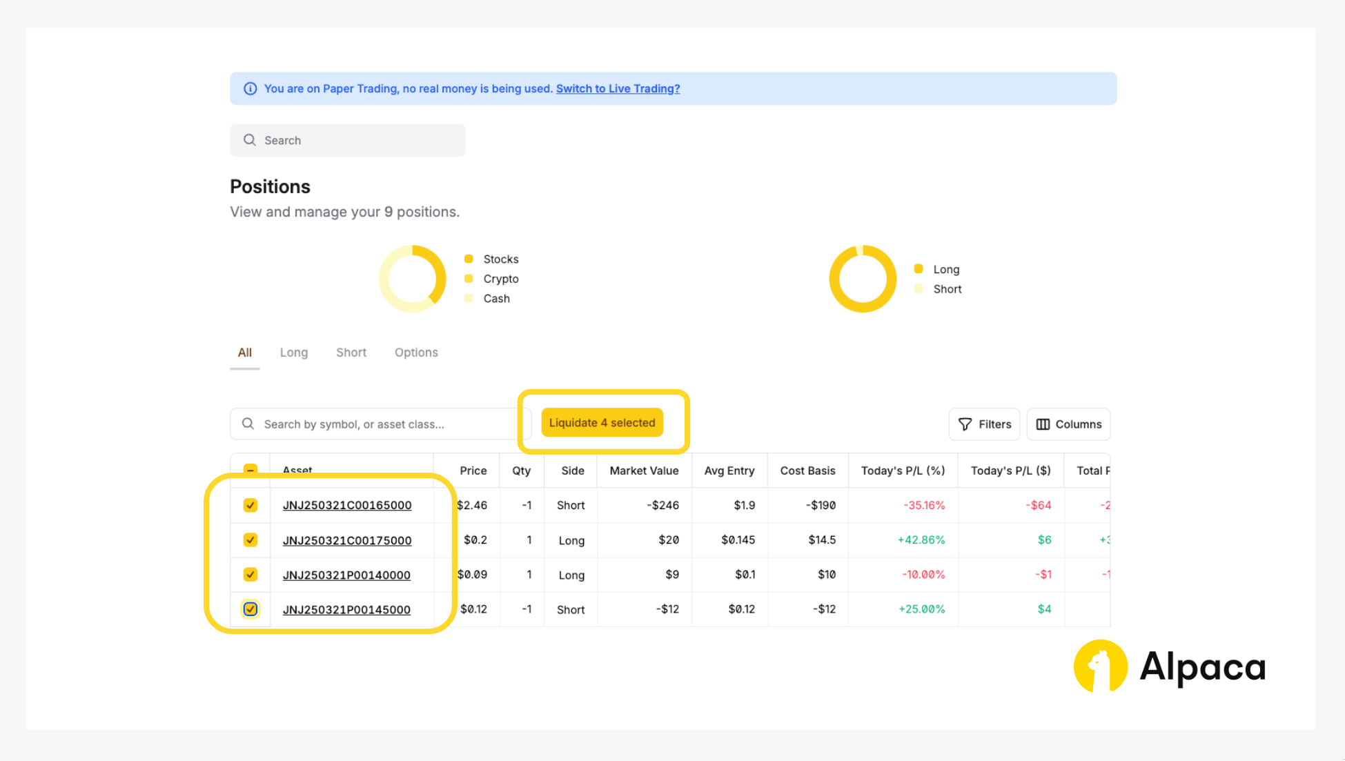
You will, then, click the “Confirm” button to liquidate the position.

Conclusion

The iron condor options strategy offers traders a structured approach to potentially profit from stable market conditions. By combining a put spread and a call spread, this strategy aims to capitalize on time decay and change in volatility, while clearly defining both potential profits and losses.

Effective risk management is crucial when implementing an iron condor. Traders should thoroughly assess market conditions, select appropriate strike prices, and continuously monitor positions to make informed adjustments as needed. It's important to recognize that, like all trading strategies, the iron condor does not guarantee profits and carries inherent risks.

Continuous learning and diligent research are essential to mastering the nuances of this strategy. Utilizing tools such as Alpaca's paper trading platform can provide valuable hands-on experience without financial exposure.

We hope you've found this tutorial on how to trade iron condor insightful and useful for getting started on your own strategy. As you put these concepts into practice, feel free to share your feedback and experiences on our forum, Slack community, or subreddit! And don’t forget to check out the rest of our options-related tutorials.

Interested in learning more about options trading with Alpaca’s Trading API? Here are some resources:

• Sign up for an Alpaca Trading API account
• How to Connect to Alpaca's Trading API
• How to Start Paper Trading with Alpaca's Trading API
• How to Trade Options with Alpaca’s Trading API
• Read more Options Trading Tutorials
• Documentation: Options Trading

FAQs

Why does an iron condor strategy fail?

An iron condor strategy can fail if the underlying asset experiences significant price movement beyond the established strike prices, leading to potential losses. Additionally, unexpected increases in market volatility can adversely affect the position's profitability. Overconfidence in market stability and failure to adjust positions in response to changing conditions are common pitfalls. 

Is the iron condor bearish or bullish?

The iron condor is a neutral options strategy designed to profit when the underlying asset remains within a specific price range, therefore, it is neither inherently bullish nor bearish. However, traders can adjust the strike prices to introduce a slight bullish or bearish bias, depending on their market outlook. 

What is the disadvantage of an iron condor?

One primary disadvantage of an iron condor is its limited profit potential, as maximum gains are capped by the net premium received. Additionally, while losses are theoretically limited, significant price movements in the underlying asset can lead to substantial losses relative to the potential gains. The strategy also requires careful monitoring and adjustments, as unexpected market volatility can impact its effectiveness.

Options trading is not suitable for all investors due to its inherent high risk, which can potentially result in significant losses. Please read Characteristics and Risks of Standardized Options before investing in options.

Past hypothetical backtest results do not guarantee future returns, and actual results may vary from the analysis.

The Paper Trading API is offered by AlpacaDB, Inc. and does not require real money or permit a user to transact in real securities in the market. Providing use of the Paper Trading API is not an offer or solicitation to buy or sell securities, securities derivative or futures products of any kind, or any type of trading or investment advice, recommendation or strategy, given or in any manner endorsed by AlpacaDB, Inc. or any AlpacaDB, Inc. affiliate and the information made available through the Paper Trading API is not an offer or solicitation of any kind in any jurisdiction where AlpacaDB, Inc. or any AlpacaDB, Inc. affiliate (collectively, “Alpaca”) is not authorized to do business.

Please note that this article is for general informational purposes only and is believed to be accurate as of the posting date but may be subject to change. The examples above are for illustrative purposes only.

All investments involve risk, and the past performance of a security, or financial product does not guarantee future results or returns. There is no guarantee that any investment strategy will achieve its objectives. Please note that diversification does not ensure a profit, or protect against loss. There is always the potential of losing money when you invest in securities, or other financial products. Investors should consider their investment objectives and risks carefully before investing.

Securities brokerage services are provided by Alpaca Securities LLC ("Alpaca Securities"), member FINRA/SIPC, a wholly-owned subsidiary of AlpacaDB, Inc. Technology and services are offered by AlpacaDB, Inc.

This is not an offer, solicitation of an offer, or advice to buy or sell securities or open a brokerage account in any jurisdiction where Alpaca Securities are not registered or licensed, as applicable.