Understanding advanced options strategies can be challenging, especially when there are multiple contracts involved in a single trade, and this is the case with an iron butterfly. 

In this tutorial, we will explore the fundamentals of an iron butterfly options strategy, provide examples, discuss how market factors—including the Greeks—influence its performance, and outline the associated risks. We will also highlight actionable steps you can take for algorithmic integration using Alpaca's Trading API or manual trading using Alpaca’s dashboard.​

What Is An Iron Butterfly?

The iron butterfly is a defined-risk options strategy used to seek potential profit in neutral market conditions, though outcomes vary depending on market behavior and execution. It involves four options contracts across three strike prices—two at-the-money (ATM) options at the center strike, and two out-of-the-money (OTM) options at strike prices above and below the center. This structure forms a “butterfly” shape on a payoff diagram and can be constructed in either a long or short position.

The iron butterfly is known for having a tighter profit zone than the iron condor, as both the short call and put are placed at the same strike price. This allows it to collect a higher net premium, but also means a narrower range of profitability. It’s typically considered a non-directional or delta-neutral strategy because it centers around a specific target price and does not rely on strong directional movement. Traders often use it to take advantage of time decay (theta) and contractions in implied volatility (vega), both of which play key roles in maximizing potential return.

While the iron butterfly offers defined profit potential and capped risk—making it appealing to risk-conscious traders—it can be more sensitive to price fluctuations than wider-range strategies. For those seeking a similar strategy with a broader profit range, the iron condor may serve as an alternative.

Short Iron Butterfly vs Long Iron Butterfly

There are two primary variations of the iron butterfly: the short iron butterfly and the long iron butterfly. The table below shows a quick summary of the comparisons.

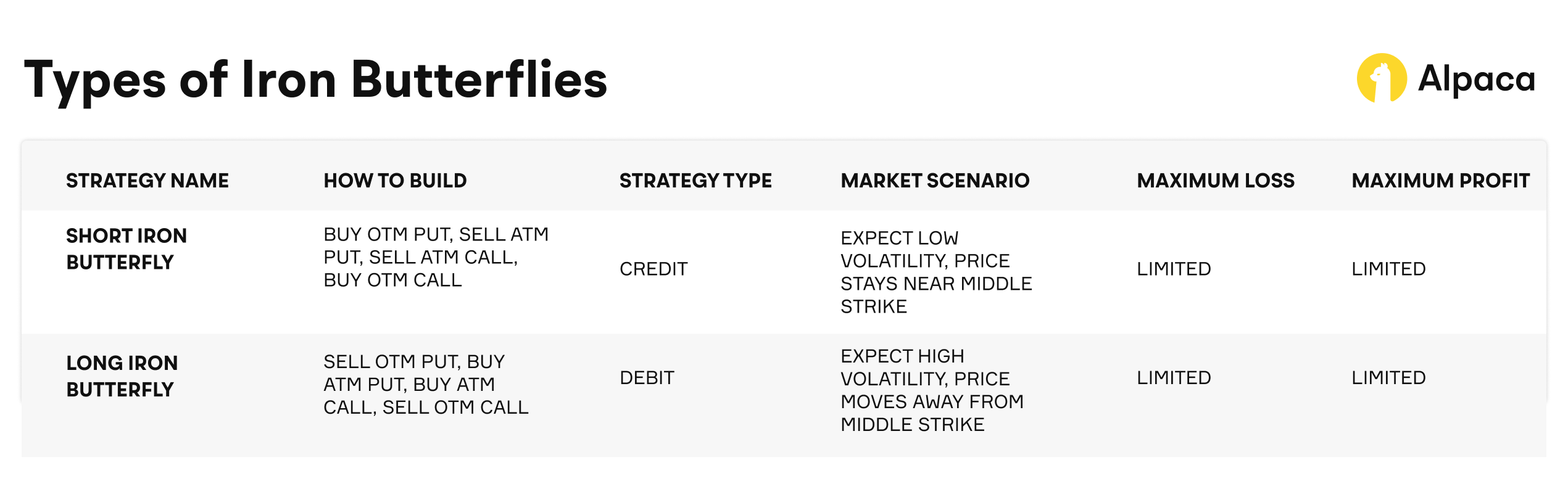
Short Iron Butterfly

A short iron butterfly is typically used by traders who anticipate a period of low volatility in the market. Rather than betting on price movement, the goal of this strategy is to potentially profit when the underlying asset stays within a narrow range. 

The short iron butterfly benefits from time decay and a decline in implied volatility, assuming the asset remains near the ATM strike. It aims to capitalize on low volatility by collecting premiums from selling options and buy it back later, hopefully for a profit, or allow it to expire worthless. However, the strategy carries the risk of losses if the price moves beyond the breakeven points.

When to Use a Short Iron Butterfly

A short iron butterfly may be considered when:

• Volatility is high but expected to decrease.
• The underlying asset is trading in a narrow range.
• A trader has a neutral outlook and anticipates price stability.

Structure (Four Legs)

To create a short iron butterfly, a trader builds the following positions — all legs share the same expiration date:

• Buy 1 OTM put (lower strike price)
• Sell 1 ATM put and 1 ATM call (at the same underlying strike price)
• Buy 1 OTM call (higher strike price)

Profit Potential

The short iron butterfly offers limited, defined profit and loss. 

• Theoretical maximum profit: It is the net credit received at entry and occurs if the underlying price settles exactly at the center strike at expiration—where all options may expire worthless.
• Theoretical maximum loss: It occurs if the underlying moves beyond either of the outer strikes and is equal to the distance between the strikes minus the credit received. Breakeven points are located at the short strike plus and minus or plus the net credit.

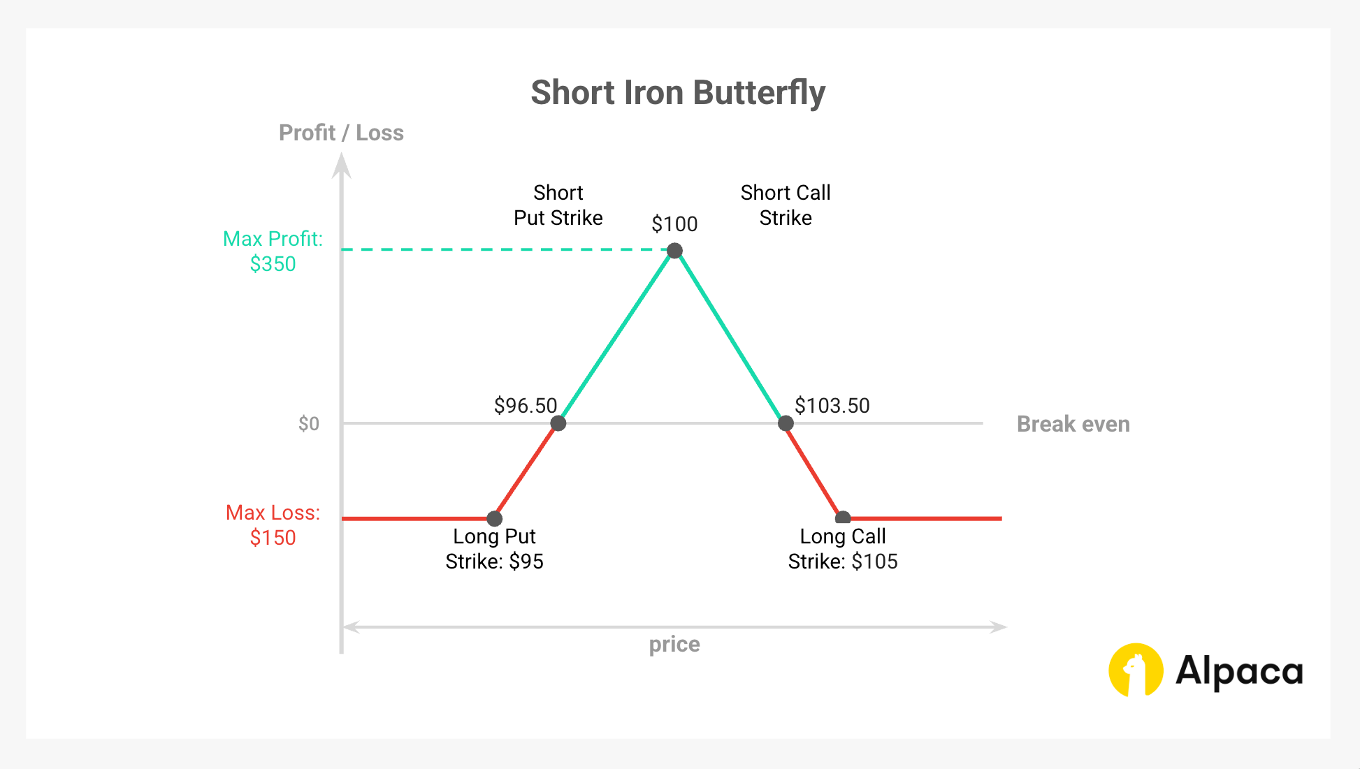
Example: Short Iron Butterfly (with payoff diagram)

Example Setup:

• Underlying Price: XYZ is trading at $100.
• Initial Credit: ($5.70 (short call) + $5.20 (short put) - $3.75 (long call) - $3.65 (long put)) x 100 = $350.00.
• Theoretical maximum profit: $350.00 (same as the initial net credit)
• Theoretical maximum Loss: ($5.00 (width of the spread (wider side)) - $3.50 (credit received)) × 100 = $150.00.
• Upper breakeven point: $100 (short call strike) + $3.50 (initial credit) = $103.50.
• Lower breakeven point: $100 (short put strike) - $3.50 (initial credit) = $96.50.

Trade Structure (Four Legs):

Scenario 1: XYZ is at $100 at expiration

• The short call and short put (both at $100) expire worthless.
• The long put ($95 strike) and long call ($105 strike) are also OTM and expire worthless.
• All options expire worthless.
• Net Profit: $350 (initial credit) – $0 (no intrinsic value) = $350 (theoretical maximum profit)

Scenario 2: XYZ is at $96.50 at expiration

• The short put ($100 strike) is in-the-money (ITM) by $3.50 = -$350
• The long put ($95 strike) is OTM and expires worthless
• The calls expire worthless
• This is the lower breakeven point
• Net Even: $350 (initial credit) – $350 (intrinsic loss on short put) = $0 (breakeven)

Scenario 3: XYZ is at $105 at expiration

• The short call ($100 strike) is ITM by $5.00 = -$500
• The long call ($105 strike) is ATM and expires worthless
• The puts are OTM and expire worthless
• Net Loss: $350 (initial credit) – $500 (loss on short call) = –$150 (theoretical maximum loss)

Note: Note: For American-style options, there's a possibility of early assignment of the short call, especially around ex-dividend dates. This can affect the strategy's outcome before the expiration date.

Long Iron Butterfly (Reverse Iron Butterfly)

The long iron butterfly is a limited-risk, limited-reward options strategy that is designed to potentially profit from significant price movement in either direction. It is typically structured as a net debit trade and benefits when the underlying asset moves sharply away from the central strike price by expiration.

When to Use a Long Iron Butterfly

This strategy may be considered when:

• Implied volatility is low at entry but expected to increase
• A strong move is anticipated in either direction, but the specific direction is uncertain
• There is a known catalyst (e.g., earnings, economic data, FDA approval) with potential for large price impact

Structure (Four Legs)

The below creates a symmetrical spread around the current price, with long protection in the center and short risk-limiting legs on the outside. The position incurs a net debit because the long options (ATM) are more expensive than the short OTM options.

• Sell 1 OTM put (lower strike price)
• Buy 1 ATM put and buy 1 ATM call (same strike price)
• Sell 1 OTM call (high strike price)

Profit and Loss Potential

• Theoretical maximum profit: Achieved when the underlying expires below the lower strike or above the upper strike, resulting in one side of the spread reaching full intrinsic value. The max profit is: Width between strikes – net debit paid
• Theoretical maximum loss: Occurs if the underlying expires exactly at the middle strike (where both long options expire worthless). Loss is limited to the net debit paid.

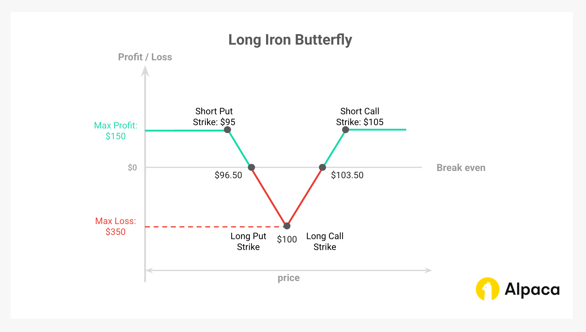
Example: Long Iron Butterfly (with payoff diagram)

Example Setup:

• Underlying Price: XYZ is trading at $100.
• Initial Debit: ($3.75 (short call) + $3.65 (short put) - $5.70 (long call) - $5.20 (long put)) x 100 = -$350.00.
• Theoretical maximum profit: ($5.00 (width of the spread (wider side)) - $3.50 (initial debit)) × 100 = $150.00.
• Theoretical maximum Loss: $350.00 (same as the initial net debit).
• Upper breakeven point: $100 (the long call strike) + $3.50 (initial debit) = $103.50.
• Lower breakeven point: $100 (the long put strike) - $3.50 (initial debit) = $96.50.

Trade Structure (Four Legs):

Scenario 1: XYZ is at $100 at expiration

• The long call and long put (both at $100) expire worthless
• The short put ($95) and short call ($105) also expire worthless
• No intrinsic value on any leg
• Net Loss: -$350 (initial debit) = Theoretical maximum loss

Scenario 2: XYZ is at $96.50 or $101.50 at expiration

• At $96.50: The $100 put is ITM by $3.50, others expire worthless
• At $103.50: The $100 call is ITM by $3.50, others expire worthless
• In both cases, the intrinsic value offsets the cost of entry
• Net Even: $350 (intrinsic gain) – $350 (initial debit) = Break-even

Scenario 3: XYZ is at $105 at expiration

• The $100 call is ITM by $5.00 = $500
• The $105 call is ATM and expires worthless
• Puts expire worthless
• Net Profit: $500 – $0 – $350 = $150 (theoretical maximum profit)

Note: Note: For American-style options, there's a possibility of early assignment of the short call, especially around ex-dividend dates. This can affect the strategy's outcome before the expiration date.

Iron Condor vs Iron Butterfly

The iron butterfly shares similarities with the iron condor but differs in structure and risk profile. We may want to fully understand the theoretical differences between the two in this iron condor vs iron butterfly comparison.

Below is a concise comparison table highlighting the key differences between the iron condor and the iron butterfly.

Understanding the Greeks for an Iron Butterfly

Options traders use the Greeks to quantify risk and price behavior. Understanding how option Greeks impact an iron butterfly is crucial for effective risk management. Here, we cover the four main Greeks.

Short Iron Butterfly

Delta

• The position is delta-neutral at initiation due to its symmetrical structure around the ATM strike.
• As the underlying moves away from the center strike, net delta becomes increasingly positive or negative, depending on direction.
• This introduces directional exposure, especially as expiration nears or the stock drifts toward a wing.

Gamma

• Gamma is low when the position is opened, limiting large delta swings.
• As expiration approaches, gamma increases, particularly near the breakeven points.
• Higher gamma near expiration increases sensitivity to small price movements, requiring more frequent monitoring.

Theta

• The short iron butterfly benefits from positive theta, as the position collects net premium.
• Time decay accelerates as expiration nears, favoring the trade if the stock stays near the center strike.
• Theta works best in stable markets where the underlying price remains range-bound.

Vega

• The position has negative vega, meaning it loses value if implied volatility rises.
• Rising volatility inflates option premiums, increasing the value of the short legs (a liability).
• Falling volatility benefits the trade by reducing premium and increasing the likelihood of expiring within the profitable zone.

Long Iron Butterfly

Delta

• The position starts delta-neutral, like the short version.
• As the stock price moves strongly in either direction, net delta becomes increasingly directional.
• Profits come when the stock breaks out beyond either wing, where delta shifts more meaningfully.

Gamma

• Gamma is low at initiation but rises near expiration.
• The effect is most pronounced when the stock approaches the strike prices of the short wing options, as these options begin to transition toward the money, resulting in a significant increase in gamma and rapid changes in delta.

Theta

• The long iron butterfly has negative theta, meaning it loses value as time passes.
• Time decay works against the position, particularly if the stock remains near the center strike.
• The strategy requires significant price movement before expiration to offset this decay.

Vega

• The position carries positive vega, meaning it benefits from rising implied volatility.
• Higher volatility expands premiums and increases the value of the long options.
• Declining volatility can hurt the position by reducing extrinsic value.

Risk Management and Considerations

Early Assignment Risk

Even though early assignment is uncommon, American-style options can be assigned before expiration—especially if a short option becomes deeply ITM. This risk is higher near ex-dividend dates or just before expiration, which can lead to unwanted exposure or early use of margin. Traders typically manage this risk by monitoring the option’s sensitivity and remaining time value, and may choose to close or roll the position before expiration.

Volatility Risk

Short iron butterflies are short vega, meaning they are vulnerable to unexpected increases in implied volatility. If volatility rises suddenly, the position’s value can increase, causing a paper loss for the seller—especially if the price moves close to the breakeven point. Staying aware of key news events, earnings releases, or economic announcements may possibly help reduce this risk.

Liquidity Risk

Since an iron butterfly involves four options, entering or exiting the position would require a market with good liquidity. Wide bid-ask spreads can result in extra costs and slippage, which can affect both profitability and risk. Traders usually prefer underlying assets that offer tight spreads, high open interest, and strong trading volume for smoother order execution.

Margin Requirements

Although iron butterflies have a defined theoretical maximum loss, brokers may require margin based on the full width of the spread rather than just the net credit received. Margin requirements vary by account type, broker, and market conditions. It’s important to understand how margin is calculated, especially when trading multiple contracts, to ensure proper risk management.

Execute your trading algos commission-free

Sign Up for Free

Executing a Short Iron Butterfly Using Alpaca’s Trading API

This section provides a step-by-step guide to implementing a short iron butterfly using Python and Alpaca’s Trading API in the Paper Trading environment. The strategy is a four-legged, neutral strategy that involves simultaneously selling ATM call/put options and an OTM call/put options. This approach helps manage risk and optimize decision-making by leveraging key metrics and filters.

Important Notes:

• The following code assumes a flat interest rate, ignores dividends, is not optimized for 0DTE options, and does not account for market hours. It serves as a starting point, not a fully developed strategy.
• On expiration day, Alpaca enforces an early order submission cutoff:
  • 3:15 p.m. ET for stocks and most options
  • 3:30 p.m. ET for broad-based ETFs (e.g., SPY, QQQ)
  • Any orders submitted after these times will be automatically rejected.
  • Expiring positions are auto-liquidated starting at 3:30 p.m. ET (stocks/options) and 3:45 p.m. ET (broad-based ETFs) for risk management.
• For multi-leg (MLeg) orders, all legs, covering each other, must be included within the same order for acceptance. This is especially relevant for strategies involving potential uncovered short options, such as short put calendar spreads and short call calendar spreads, which require option level 4 approval. Please refer to Alpaca's multi-leg order restrictions for details on uncovered legs.

Example stock "JNJ" is used for demonstration purposes and should not be considered investment advice.

Step 1: Setting Up the Environment and Trade Parameters

The first step involves configuring the environment for trading a short iron butterfly and specifying your Alpaca Paper Trading API keys. This ensures your API connections and variable setup are secure and streamlined for data retrieval and trading in operations. 

Note: While we are using Jupyter Notebook for this tutorial, you can use Google Collab or any other IDE as your code environment. You can also find all of the below code on Alpaca’s Github page.

# Install or upgrade the package `alpaca-py` and import it
!python3 -m pip install --upgrade alpaca-py

import pandas as pd
import numpy as np
import alpaca
import time
from datetime import datetime, timedelta
from zoneinfo import ZoneInfo
from alpaca.data.timeframe import TimeFrame, TimeFrameUnit
from dotenv import load_dotenv
import os
from typing import Any, Dict, List, Optional, Tuple

from alpaca.data.historical.option import OptionHistoricalDataClient
from alpaca.data.historical.stock import StockHistoricalDataClient, StockLatestTradeRequest
from alpaca.data.requests import StockBarsRequest, OptionSnapshotRequest, OptionBarsRequest
from alpaca.trading.client import TradingClient
from alpaca.trading.requests import (
    MarketOrderRequest,
    GetOptionContractsRequest,
    MarketOrderRequest,
    OptionLegRequest,
    ClosePositionRequest,
)
from alpaca.trading.enums import (
    AssetStatus,
    ExerciseStyle,
    OrderSide,
    OrderClass,
    OrderStatus,
    OrderType,
    TimeInForce,
    QueryOrderStatus,
    ContractType,
)

The script initializes Alpaca clients for trading stocks and options, as well as for handling data requests.

# API credentials for Alpaca
API_KEY = "YOUR_ALPACA_API_KEY_FOR_PAPER_TRADING"
API_SECRET = 'YOUR_ALPACA_API_SECRET_KEY_FOR_PAPER_TRADING'
BASE_URL = None
## We use paper environment for this example (Please do not modify this. This example is for paper trading only)
PAPER = True

# Initialize Alpaca clients
trade_client = TradingClient(api_key=API_KEY, secret_key=API_SECRET, paper=PAPER, url_override=BASE_URL)
option_historical_data_client = OptionHistoricalDataClient(api_key=API_KEY, secret_key=API_SECRET, url_override=BASE_URL)
stock_data_client = StockHistoricalDataClient(api_key=API_KEY, secret_key=API_SECRET)

# Below are the variables for development this documents
# Please do not change these variables
trade_api_url = None
trade_api_wss = None
data_api_url = None
option_stream_data_wss = None

Step 2: Pick Your Strategy Inputs: Risk Management and Position Sizing

For an algorithmic short iron butterfly, selecting the right strategy inputs is crucial to managing risk and sizing positions effectively. These inputs ensure each trade meets predetermined risk/reward criteria and fits within your overall portfolio limits.

Liquidity and Open Interest Threshold

To avoid thinly traded options and wide bid-ask spreads, a minimum open interest threshold (e.g., 50) is set. This filter ensures only contracts with robust market participation are considered, leading to smoother execution and more reliable pricing.

Option Greeks and IV Ranges

Choosing the right options involves filtering by key risk measures. For a short iron butterfly, traders require all four legs to meet specific criteria—such as having an expiration between 7 and 42 days. Entry is favored when the underlying's implied volatility rank is elevated (e.g., >50%-70%). The goal is delta neutrality (net delta ≈ 0.0) for the overall position. These choices result in a position with specific Greek characteristics, typically positive Theta (e.g., +0.08 to +0.20), influencing sensitivity to time decay, volatility changes, and price movements.

Target Profit

A clear profit target is essential. By setting a target profit percentage (e.g., 60%), the option strategy is closed once its value moves in your favor by that amount. This predefined exit may help to secure gains and minimizes the risk of losing accrued profits due to market reversals.

Buying Power Allocation

Limiting capital exposure is another key element. Traders typically allocate around 2-5% of total buying power to any single trade. This dynamic calculation keeps risk consistent across trades, ensuring that even adverse moves have a limited impact on the overall account.

Evaluating the Cost

Cost evaluation involves setting an acceptable strike range relative to the underlying price. A common method is to define strikes within a fixed percentage (such as ±10%) of the current price. This approach balances potential profit with manageable risk. Incorporating a risk-free rate (typically 1%) into the calculations refines the estimation of the Greeks and IV, resulting in a more accurate assessment of the trade’s risk/reward profile.

Monitoring and Potential Adjustments

Active monitoring is essential once the trade is live. Predefined thresholds for adjustments—such as exit triggers if delta or IV move beyond set limits (e.g., net delta above 0.50 or net IV rising to 60%)—allow traders to roll or exit positions promptly. These dynamic controls help maintain the desired risk profile during volatile periods.

Liquidity Considerations and Stop-Loss Limits

Beyond open interest filters for all four legs, short iron butterfly risk is managed structurally by wing width (short-to-long strike distance), defining theoretical max loss. Stop-loss orders safeguard against adverse moves, perhaps triggered if price nears the long strikes or if total position loss hits a set limit. Slippage on stop orders remains a concern in fast markets, especially with multi-leg positions.

# Select the underlying stock (Johnson & Johnson)
underlying_symbol = 'JNJ'

# Set the timezone
timezone = ZoneInfo('America/New_York')

# Get current date in US/Eastern timezone
today = datetime.now(timezone).date()

# Define a 10% range around the underlying price. 
STRIKE_RANGE = 0.10

# Buying power percentage to use for the trade
BUY_POWER_LIMIT = 0.05

# Risk free rate for the options greeks and IV calculations
risk_free_rate = 0.01

# Check account buying power
buying_power = float(trade_client.get_account().buying_power)

# Set the open interest volume threshold
OI_THRESHOLD = 50

# Calculate the limit amount of buying power to use for the trade
buying_power_limit = buying_power * BUY_POWER_LIMIT

# Set the expiration date range for the options
min_expiration = today + timedelta(days=7)
max_expiration = today + timedelta(days=42)

# Get the latest price of the underlying stock
def get_underlying_price(symbol):
    # Get the latest trade for the underlying stock
    underlying_trade_request = StockLatestTradeRequest(symbol_or_symbols=symbol)
    underlying_trade_response = stock_data_client.get_stock_latest_trade(underlying_trade_request)
    return underlying_trade_response[symbol].price

# Get the latest price of the underlying stock
underlying_price = get_underlying_price(underlying_symbol)

# Set the minimum and maximum strike prices based on the underlying price
min_strike = str(underlying_price * (1 - STRIKE_RANGE))
max_strike = str(underlying_price * (1 + STRIKE_RANGE))

# Each key corresponds to a leg and maps to a tuple of: (expiration range, IV range, delta range, theta range)
criteria = {
    'long_put':  ((14, 35), (0.10, 0.40), (-0.40, -0.10), (-0.1, -0.005)),
    'short_put': ((14, 35), (0.15, 0.50), (-0.60, -0.30), (-0.15, -0.01)),
    'short_call':((14, 35), (0.15, 0.50), (0.60, 0.30), (-0.15, -0.01)),
    'long_call': ((14, 35), (0.10, 0.40), (0.40, 0.10), (-0.1, -0.005))
}

# Set target profit levels
TARGET_PROFIT_PERCENTAGE = 0.60
DELTA_STOP_LOSS = 0.50
IV_STOP_LOSS = 0.60

# Display the values
print(f"Underlying Symbol: {underlying_symbol}")
print(f"{underlying_symbol} price: {underlying_price}")
print(f"Buying Power Limit: {buying_power_limit}")
print(f"Minimum Expiration Date: {min_expiration}")
print(f"Maximum Expiration Date: {max_expiration}")
print(f"Minimum Strike Price: {min_strike}")
print(f"Maximum Strike Price: {max_strike}")

Step 3: Market Data Analysis with Underlying Assets

When implementing a short iron butterfly, it's essential to identify market conditions that support the strategy. Using a combination of price trends, volatility measures, and technical indicators, traders would be able to optimize entry points and improve trade efficiency. The following factors may help a short iron butterfly setup based on underlying asset price movement and volatility events.

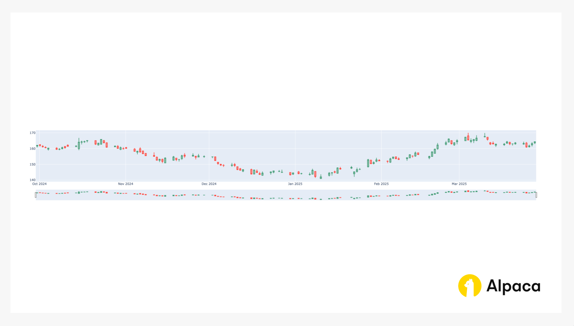
Stock Price Trends (Bar Chart Analysis)

Monitoring historical price movements can help traders evaluate the broader trend of the underlying asset before entering a short iron butterfly. Reviewing candlestick charts offers valuable insights into recent price action, as well as key support and resistance levels. This analysis helps traders identify whether the asset is trending upward or trading within a range.

A short iron butterfly spread's theoretical maximum profit occurs when the stock price equals the center strike price at expiration. Depending on the stock price's relation to the center strike price when the position is established, the forecast can be "neutral," "modestly bullish," or "modestly bearish."

# Get the historical data for the underlying stock by symbol and timeframe
# ref. https://alpaca.markets/sdks/python/api_reference/data/option/historical.html
def get_stock_data(underlying_symbol, days=90):
    today = datetime.now(timezone).date()
    req = StockBarsRequest(
        symbol_or_symbols=[underlying_symbol],
        timeframe=TimeFrame(amount=1, unit=TimeFrameUnit.Day),     # specify timeframe
        start=today - timedelta(days=days),                          # specify start datetime, default=the beginning of the current day.
    )
    return stock_data_client.get_stock_bars(req).df

# List of stock agg objects while dropping the symbol column
priceData = get_stock_data(underlying_symbol, days=180).reset_index(level='symbol', drop=True)

import plotly.graph_objects as go

# Bar chart for the stock price
fig = go.Figure(data=[go.Candlestick(x=priceData.index,
                open=priceData['open'],
                high=priceData['high'],
                low=priceData['low'],
                close=priceData['close'])])

fig.show()

This code returns the bar chart like in the image below.

Bollinger Bands for Volatility Assessment

Bollinger Bands provide a dynamic range around the asset's price, helping traders assess current market volatility and potential price extremes. When the underlying stock price approaches the upper Bollinger Band, it may indicate overbought conditions, while a move toward the lower band could suggest oversold levels.

For a short iron butterfly, Bollinger Bands can help assess if the asset is exhibiting price stability and low volatility, conditions often sought for this strategy. A price trading calmly between the bands, ideally with the bands narrowing, may signal conditions where the stock could remain near the central short strike price. In contrast, if the asset is persistently hitting the upper or lower band or the bands are widening (indicating strong trends or increasing volatility), the strategy’s chances of success may decline, as sharp trends or unpredictable price swings increase the risk of the price moving significantly away from the short strike, potentially causing losses.

# setup bollinger band calculations
def check_bb(df, period=14, multiplier=2):
    bollinger_bands = []
    # Calculate the Simple Moving Average (SMA)
    df['SMA'] = df['close'].rolling(window=period).mean()
    # Calculate the rolling standard deviation
    df['StdDev'] = df['close'].rolling(window=period).std()
    # Calculate the Upper Bollinger Band (two standard deviation)
    df['Upper Band'] = df['SMA'] + (multiplier * df['StdDev'])
    # Calculate the Lower Bollinger Band (two standard deviation)
    df['Lower Band'] = df['SMA'] - (multiplier * df['StdDev'])
    # Get the most recent Upper Band value
    upper_bollinger_band = df['Upper Band'].iloc[-1]
    lower_bollinger_band = df['Lower Band'].iloc[-1]
    
    bollinger_bands = [upper_bollinger_band, lower_bollinger_band]
    return bollinger_bands

bollinger_bands = check_bb(priceData, 14, 2)

print(f"Latest Upper Bollinger Band is: {bollinger_bands[0]}. Latest Lower Bollinger Band is {bollinger_bands[1]}; while underlying stock '{underlying_symbol}' price is {underlying_price}.")

Step 4: Set up for a Short Iron Butterfly (Find four option legs)

This code sets up a tool for printing messages from the code. It tells Python to show general messages (INFO level) and more detailed messages (DEBUG level) so we can see what's happening and troubleshoot if needed.

# Configure logging
import logging
logging.basicConfig(level=logging.INFO)
logger = logging.getLogger(__name__)
logger.setLevel(logging.DEBUG)

The get_options function retrieves active option contracts for a specified underlying symbol within a given strike price and expiration date range. Reminder to specify option_type as either ContractType.CALL or ContractType.PUT to filter for the desired option type.

# option_type: ContractType.CALL or ContractType.PUT.
def get_options(underlying_symbol, min_strike, max_strike, min_expiration, max_expiration, option_type):
    req = GetOptionContractsRequest(
        underlying_symbols=[underlying_symbol],
        status=AssetStatus.ACTIVE,
        type=option_type,
        strike_price_gte=min_strike,
        strike_price_lte=max_strike,
        expiration_date_gte=min_expiration,
        expiration_date_lte=max_expiration,        
    )
    return trade_client.get_option_contracts(req).option_contracts

The helper function validate_sufficient_OI verifies that an option's data includes the necessary fields and that its open interest exceeds a specified threshold. It is used at the start of the workflow to ensure that only eligible options are processed further.

def validate_sufficient_OI(option_data, OI_THRESHOLD):
    '''Ensure that the option has the required fields and sufficient open interest.'''
    if option_data.open_interest is None or option_data.open_interest_date is None:
        return False
    if float(option_data.open_interest) <= OI_THRESHOLD:
        return False
    return True

The calculate_option_metrics computes essential metrics for an option contract by retrieving current market data and calculating relevant values. Here’s what it does:

1. Determine Expiration Details:
   • It extracts the option’s expiration date from the provided data.
   • It calculates the number of days remaining until expiration by comparing the expiration date with the current date.
2. Retrieve Latest Market Data via Alpaca’s API:
   • The function constructs an OptionSnapshotRequest—a method provided by Alpaca’s API—using the option’s symbol.
   • It then calls option_historical_data_client.get_option_snapshot() to fetch a snapshot of the latest market data for that option.
3. Validate Snapshot Data: 
   • It checks if the fetched market data (snapshot) or essential parts like the latest quote (snapshot.latest_quote) or Greeks data (snapshot.greeks) are missing (None). If any crucial data is unavailable, the function stops early and returns None to indicate it couldn't proceed.
4. Calculate the Option Price:
   • The mid-price is calculated as the average of the bid and ask prices obtained from the snapshot’s latest quote.
5. Extract Implied Volatility and Greeks:
   • The implied volatility (IV) is directly extracted from the snapshot.
   • Key option Greeks—delta, gamma, theta, and vega—are also extracted from the snapshot for further risk and pricing analysis.
6. Return Metrics:
   • Finally, the function returns a dictionary containing the calculated option price, expiration date, remaining days, IV, and the Greeks for use in other parts of the trading strategy.

Note: Although the function accepts parameters for underlying_price and risk_free_rate, these are not utilized in the current calculations.

def calculate_option_metrics(option_data, underlying_price, risk_free_rate):
    """
    Calculate key option metrics including option price, implied volatility (IV), and option Greeks.
    """
    
    # Calculate expiration and remaining days
    option_symbol = option_data['symbol']
    expiration_date = pd.Timestamp(option_data['expiration_date'])
    remaining_days = (expiration_date - pd.Timestamp.now()).days
    
    # Retrieve the latest quote for the option
    req = OptionSnapshotRequest(symbol_or_symbols = option_symbol)
    snapshot = option_historical_data_client.get_option_snapshot(req)[option_symbol]

    # Check if snapshot or its required attributes are None; if so, skip further processing
    if snapshot is None or snapshot.latest_quote is None or snapshot.greeks is None:
        return None
    
    option_price = (snapshot.latest_quote.bid_price + snapshot.latest_quote.ask_price) / 2

    ## implied volatility
    iv = snapshot.implied_volatility
    ## Greeks
    delta = snapshot.greeks.delta
    gamma = snapshot.greeks.gamma
    theta = snapshot.greeks.theta
    vega = snapshot.greeks.vega
    
    return {
        'option_price': option_price,
        'expiration_date': expiration_date,
        'remaining_days': remaining_days,
        'iv': iv,
        'delta': delta,
        'gamma': gamma,
        'theta': theta,
        'vega': vega
    }

This function ensures that the provided option_data is in dictionary format. If option_data is given in a different format (e.g. OptionContract object), it converts it to a dictionary.

def ensure_dict(option_data):
    """
    Convert option_data to a dict using model_dump() if available (for Pydantic models),
    otherwise return the data as-is.
    """
    if hasattr(option_data, "model_dump"):
        return option_data.model_dump()
    return option_data

The build_option_dict function builds a comprehensive option dictionary by merging the raw option data with the calculated metrics from calculate_option_metrics. It first converts the input to a dictionary using ensure_dict, then obtains all necessary metrics (like option price, IV, delta, and vega). Finally, it constructs and returns a candidate dictionary that includes both the original option details (such as id, name, symbol, strike price, etc.) and the calculated metrics. This consolidated dictionary can be used for further processing or trading decisions. If any crucial data (such as option Greeks and IV) from the calculate_option_metrics function is unavailable, the function stops early and returns None to indicate it couldn't proceed.

def build_option_dict(option_data, underlying_price, risk_free_rate):
    """
    Build an option dictionary by merging raw option data with calculated metrics.
    """
    
    option_data = ensure_dict(option_data)  # Convert to dict if necessary
    metrics = calculate_option_metrics(option_data, underlying_price, risk_free_rate)
    
    # Check if metrics is None (e.g., missing IV/Greeks); if so, skip candidate building 
    if metrics is None:
        return None
    
    candidate = {
        'id': option_data['id'],
        'name': option_data['name'],
        'symbol': option_data['symbol'],
        'strike_price': option_data['strike_price'],
        'root_symbol': option_data['root_symbol'],
        'underlying_symbol': option_data['underlying_symbol'],
        'underlying_asset_id': option_data['underlying_asset_id'],
        'close_price': option_data['close_price'],
        'close_price_date': option_data['close_price_date'],
        'expiration_date': metrics['expiration_date'],
        'remaining_days': metrics['remaining_days'],
        'open_interest': option_data['open_interest'],
        'open_interest_date': option_data['open_interest_date'],
        'size': option_data['size'],
        'status': option_data['status'],
        'style': option_data['style'],
        'tradable': option_data['tradable'],
        'type': option_data['type'],
        'initial_IV': metrics['iv'],
        'initial_delta': metrics['delta'],
        'initial_gamma': metrics['gamma'],
        'initial_theta': metrics['theta'],
        'initial_vega': metrics['vega'],
        'initial_option_price': metrics['option_price'],
    }
    
    return candidate

The function check_greeks_iv_for_candidate_option checks if a candidate option meets the filtering criteria provided as a tuple (expiration range, IV range, delta range, theta range). It is used within the main workflow to determine whether a candidate qualifies for a specific leg of a short iron butterfly.

def check_greeks_iv_for_candidate_option(candidate: Dict[str, Any], criteria: Tuple, label: str) -> bool:
    """
    Check whether a candidate option meets the filtering criteria.
    The criteria is a tuple of (expiration_range, iv_range, delta_range, theta_range).
    Logs detailed information if a candidate fails a criterion.
    """
    expiration_range, iv_range, delta_range, theta_range = criteria

    if not (expiration_range[0] <= candidate['remaining_days'] <= expiration_range[1]):
        logger.debug(f"{candidate['symbol']} fails expiration condition for {label}: remaining_days {candidate['remaining_days']} not in {expiration_range}.")
        return False
    if not (iv_range[0] <= candidate['initial_IV'] <= iv_range[1]):
        logger.debug(f"{candidate['symbol']} fails IV condition for {label}: initial_IV {candidate['initial_IV']} not in {iv_range}.")
        return False
    if not (delta_range[0] <= candidate['initial_delta'] <= delta_range[1]):
        logger.debug(f"{candidate['symbol']} fails delta condition for {label}: initial_delta {candidate['initial_delta']} not in {delta_range}.")
        return False
    if not (theta_range[0] <= candidate['initial_theta'] <= theta_range[1]):
        logger.debug(f"{candidate['symbol']} fails theta condition for {label}: initial_theta {candidate['initial_theta']} not in {theta_range}.")
        return False

    return True

The function find_nearest_strike_contract selects the contract from a list (contracts) whose strike has the minimum absolute difference from a target_price. It iterates through the list, compares strike distances to the target, and returns the single closest matching contract element, or None if the list is empty.

# This is a function that will return a contract which minimizes the difference from a target price
def find_nearest_strike_contract(contracts, target_price):
    min_diff = float('inf')
    min_contract = None

    if not contracts: # Handle empty list case
        return None
    
    for contract in contracts:
        strike = float(contract['strike_price'])
        diff = abs(strike - target_price)

        # Check if this contract is closer than the current minimum
        # No need for 'min_contract is None' check if min_diff starts at infinity
        if diff < min_diff:
            min_diff = diff
            min_contract = contract

    return min_contract

The pair_short_iron_butterfly_candidates function identifies a valid short iron butterfly combination by first locating the nearest ATM short put (atm_sp) and short call (atm_sc) relative to the underlying_price, then pairing them with suitable OTM long put (lp) and long call (lc) candidates from provided lists. It ensures the strikes follow the required order (lp strike < atm_sp strike <= atm_sc strike < lc strike), matching the typical setup for this strategy with an ATM short body and OTM protective wings. The first valid four-leg combination (lp, atm_sp, atm_sc, lc) found is returned, or (None, None, None, None) if no suitable set exists.

def pair_short_iron_butterfly_candidates(long_puts: List[Dict[str, Any]], short_puts: List[Dict[str, Any]], short_calls: List[Dict[str, Any]], long_calls: List[Dict[str, Any]], underlying_price: float) -> Tuple[Optional[Dict[str, Any]], Optional[Dict[str, Any]]]:
    """
    Returns:
        A tuple (lp, atm_sp, atm_sc, lc) of the first valid combination found,
        or (None, None, None, None) if no valid combination is found.
    """

    # Find the at-the-money (ATM) options for short put and short call contracts (returns option contract which is closest to the underlying price)
    atm_sp = find_nearest_strike_contract(short_puts, underlying_price)
    atm_sc = find_nearest_strike_contract(short_calls, underlying_price)

    # If either ATM contract wasn't found, we cannot proceed.
    if atm_sp is None or atm_sc is None:
        # Minimal logging for this failure case (optional, but helpful)
        logger.info("Could not find necessary ATM short put or short call; cannot form butterfly.")
        return None, None, None, None
        
    # Iterate through potential wings (long puts and long calls)
    for lp in long_puts:
        for lc in long_calls:
            if (lp['strike_price'] < atm_sp['strike_price']) and (atm_sp['strike_price'] <= atm_sc['strike_price']) and (atm_sc['strike_price'] < lc['strike_price']):
                logger.info(f"Selected short iron butterfly: long_put {lp['symbol']}; short_put {atm_sp['symbol']}; short_call {atm_sc['symbol']}; long_call {lc['symbol']} with expiration {lc['expiration_date']}.")
                return lp, atm_sp, atm_sc, lc
    
    # If the loops complete without finding a suitable long put/call pair for the ATM body
    logger.info(f"No valid short iron butterfly pair found for expiration {lc['expiration_date']}: "
                f"Found ATM body (SP@{atm_sp['strike_price']}/SC@{atm_sc['strike_price']}) "
                f"but no suitable OTM wings (LP/LC) found in candidate lists.")
  
    return None, None, None, None

This check_risk_and_buying_power function calculates the theoretical maximum loss (risk) of a short iron butterfly and ensures it does not exceed the buying power limit. It compares the difference between the short options’ prices and the long options’ prices, subtracted by the initial credit and multiplied by the contract size. If the cost is too high, it raises an exception to prevent the trade.

def check_risk_and_buying_power(long_put: Dict[str, Any], short_put: Dict[str, Any], short_call: Dict[str, Any], long_call: Dict[str, Any], buying_power_limit: float) -> None:
    """
    Calculates the width of the spread minus the credit received for a short iron butterfly and checks it against the buying power limit.
    If the buying power requirement is not met, the exception is thrown and the rest of the code is never executed.
    """
    option_size = float(short_put['size'])
    premium_received = short_put['initial_option_price'] + short_call['initial_option_price'] - long_put['initial_option_price'] - long_call['initial_option_price']
    # Determine the wider spread width
    spread_width = max(short_put['strike_price'] - long_put['strike_price'], long_call['strike_price'] - short_call['strike_price'])
    # Calculate the risk
    risk = (spread_width - premium_received) * option_size
    logger.info(f"Calculated short iron butterfly risk: {risk}.")
    
    if risk >= buying_power_limit:
        raise Exception('Buying power limit exceeded for a short iron butterfly risk.')

The find_options_for_short_iron_butterfly function orchestrates the process of identifying and validating a short iron butterfly spread from input put and call lists. 

Here’s its workflow:

• Initialize & Prepare: Creates dictionaries to group potential candidates by leg type (long/short put/call) and expiration date. It then combines the input put/call lists for unified processing.
• Filter, Process & Group Candidates: Iterates through all options: filters by open interest (validate_sufficient_OI), builds a candidate record with metrics (build_option_dict), checks against leg-specific criteria (check_greeks_iv_for_candidate_option), and groups qualifying candidates by expiration and leg type. Options failing any step are skipped.
• Identify Viable Expirations: Determines and sorts the common expiration dates that possess potential candidates for all four required butterfly legs.
• Attempt Pairing & Validation: Loops through the viable expiration dates: retrieves the four candidate lists, attempts to find a structurally valid four-leg combination using pair_short_iron_butterfly_candidates, and if successful, validates the combination against risk limits using check_risk_and_buying_power.
• Return Result: Returns the first four-leg combination [lp, sp, sc, lc] that passes all structural and risk checks. If no suitable spread is found across all viable expirations, it returns [None, None, None, None].

def find_options_for_short_iron_butterfly(put_options, call_options, underlying_price, risk_free_rate, buying_power_limit, criteria, OI_THRESHOLD):
    """
    Refactored workflow to find and validate short iron butterfly candidates.
    Processes puts and calls in a single loop, groups by expiration, filters by OI and criteria, pairs candidates, checks risk, and returns the first valid set.

    Returns:
        A list containing four dictionaries [long_put, short_put, short_call, long_call]
        representing the selected legs if a valid combination is found,
        otherwise an empty list ([]).
    """
    short_put_candidates_by_exp: Dict[pd.Timestamp, List[Dict[str, Any]]] = {}
    long_put_candidates_by_exp: Dict[pd.Timestamp, List[Dict[str, Any]]] = {}
    short_call_candidates_by_exp: Dict[pd.Timestamp, List[Dict[str, Any]]] = {}
    long_call_candidates_by_exp: Dict[pd.Timestamp, List[Dict[str, Any]]] = {}
    
    # Combine puts and calls with their type for single processing loop
    # This assumes put_options and call_options are lists/iterables
    all_options_with_type = [('put', opt) for opt in put_options] + [('call', opt) for opt in call_options]
    logger.info(f"Starting processing for {len(all_options_with_type)} total options...")

    for option_type, option_data in all_options_with_type:
        # 1. Common Step: Check Open Interest
        if not validate_sufficient_OI(option_data, OI_THRESHOLD):
            logger.warning(f"Insufficient OI for {getattr(option_data, 'symbol', 'unknown')}. Skipping.") # Optional logging
            continue

        # 2. Common Step: Build Candidate Dictionary
        candidate = build_option_dict(option_data, underlying_price, risk_free_rate)
        # Skip if candidate creation fails (e.g., missing IV/Greeks)
        if candidate is None:
            continue
        expiration_date = candidate['expiration_date']

        # 3. Grouping & Categorization (based on option_type)
        # Appends candidates to the original separate dictionaries
        if option_type == 'put':
            short_put_candidates_by_exp.setdefault(expiration_date, [])
            long_put_candidates_by_exp.setdefault(expiration_date, [])
            if check_greeks_iv_for_candidate_option(candidate, criteria.get('short_put', {}), 'short_put'):
                short_put_candidates_by_exp[expiration_date].append(candidate)
            if check_greeks_iv_for_candidate_option(candidate, criteria.get('long_put', {}), 'long_put'):
                long_put_candidates_by_exp[expiration_date].append(candidate)
        elif option_type == 'call':
            short_call_candidates_by_exp.setdefault(expiration_date, [])
            long_call_candidates_by_exp.setdefault(expiration_date, [])
            if check_greeks_iv_for_candidate_option(candidate, criteria.get('short_call', {}), 'short_call'):
                short_call_candidates_by_exp[expiration_date].append(candidate)
            if check_greeks_iv_for_candidate_option(candidate, criteria.get('long_call', {}), 'long_call'):
                long_call_candidates_by_exp[expiration_date].append(candidate)
    
    # Process only expiration dates common to all four candidate groups
    logger.info("Finding common expirations and attempting pairing...")
    common_expirations = set(short_put_candidates_by_exp.keys()) & set(long_put_candidates_by_exp.keys()) & set(short_call_candidates_by_exp.keys()) & set(long_call_candidates_by_exp.keys())
    sorted_common_expirations = sorted(list(common_expirations))

    for expiration_date in sorted_common_expirations:
            logger.debug(f"Checking common expiration: {expiration_date}")

            sp_list = short_put_candidates_by_exp.get(expiration_date, [])
            lp_list = long_put_candidates_by_exp.get(expiration_date, [])
            sc_list = short_call_candidates_by_exp.get(expiration_date, [])
            lc_list = long_call_candidates_by_exp.get(expiration_date, [])

            if not all([sp_list, lp_list, sc_list, lc_list]):
                logger.warning(f"Expiration {expiration_date} in common set but found empty list(s). Skipping.")
                continue

            paired_legs_tuple = pair_short_iron_butterfly_candidates(
                long_puts=lp_list,
                short_puts=sp_list,
                short_calls=sc_list,
                long_calls=lc_list,
                underlying_price=underlying_price
            )

            if paired_legs_tuple and len(paired_legs_tuple) == 4 and all(leg is not None for leg in paired_legs_tuple):
                lp, sp, sc, lc = paired_legs_tuple # Unpack

                try:
                    check_risk_and_buying_power(lp, sp, sc, lc, buying_power_limit)
                    logger.info(f"Selected short iron butterfly for expiration {expiration_date}: long_put {lp['symbol']}, short_put {sp['symbol']}, short_call {sc['symbol']}, long_call {lc['symbol']}.")
                    # <<< Return the first valid, risk-checked pair
                    option_legs = [lp, sp, sc, lc]
                    return option_legs
                except Exception as e:
                    logger.error(f"Pair for expiration {expiration_date} failed buying power check: {e}")
                    # <<< Continue to the next expiration date
                    continue
            # else:
                # logger.debug(f"No valid 4-leg combo returned by pairing function for {expiration_date}.")

    # If loop completes without returning
    logger.info("No valid short iron butterfly found meeting all criteria.")
    option_legs = [None, None, None, None]
    return option_legs

We now can run the get_options function and the find_options_for_short_iron_butterfly function to find a reasonable set of options for a short iron butterfly.

put_options = get_options(underlying_symbol, min_strike, max_strike, min_expiration, max_expiration, ContractType.PUT)
call_options = get_options(underlying_symbol, min_strike, max_strike, min_expiration, max_expiration, ContractType.CALL)

short_iron_butterfly_order_legs = find_options_for_short_iron_butterfly(put_options, call_options, underlying_price, risk_free_rate, buying_power_limit, criteria, OI_THRESHOLD)

We can check the selected options and potential credit by the selected short iron butterfly.

# Check spread width
lp = short_iron_butterfly_order_legs[0]
sp = short_iron_butterfly_order_legs[1]
sc = short_iron_butterfly_order_legs[2]
lc = short_iron_butterfly_order_legs[3]

print(f"The width for the short iron butterfly (initial premium collected): {sp['initial_option_price'] + sc['initial_option_price'] - lp['initial_option_price'] - lc['initial_option_price']}; the initial net delta: {lc['initial_delta'] + abs(sp['initial_delta']) - abs(sc['initial_delta']) - abs(lp['initial_delta'])}")

Step 5: Execute a Short Iron Butterfly

The script below builds the list of options for a short iron butterfly and places an order.

# Place orders for the short iron butterfly spread if all options are found
if short_iron_butterfly_order_legs:
    # Create a list for the order request
    order_legs = []
    ## Append long put
    order_legs.append(OptionLegRequest(
        symbol=short_iron_butterfly_order_legs[0]["symbol"],
        side=OrderSide.SELL,
        ratio_qty=1
    ))
    ## Append short put
    order_legs.append(OptionLegRequest(
        symbol=short_iron_butterfly_order_legs[1]["symbol"],
        side=OrderSide.BUY,
        ratio_qty=1
    ))
    ## Append short call
    order_legs.append(OptionLegRequest(
        symbol=short_iron_butterfly_order_legs[2]["symbol"],
        side=OrderSide.SELL,
        ratio_qty=1
    ))
    ## Append long call
    order_legs.append(OptionLegRequest(
        symbol=short_iron_butterfly_order_legs[3]["symbol"],
        side=OrderSide.BUY,
        ratio_qty=1
    ))

    # Place the order for both legs simultaneously
    req = MarketOrderRequest(
        qty=1,
        order_class=OrderClass.MLEG,
        time_in_force=TimeInForce.DAY,
        legs=order_legs
    )
    res = trade_client.submit_order(req)
    print("Short iron butterfly order placed successfully.")

# We then check the order confirmation in detail.
res

Before the order is filled, traders may choose to cancel it. Please note that individual legs cannot be canceled or replaced. We must cancel the entire order. If you are not familiar with the level 3 option trading with multi-legs, please check out an example code for multi-leg option trading on Alpaca’s Github page

# Query by the order's id
q1 = trade_client.get_order_by_client_id(res.client_order_id)

# Replace overall order
if q1.status != OrderStatus.FILLED:
    # Cancel the whole order
    trade_client.cancel_order_by_id(res.id)
    print(f"Canceled order: {res}")

else:
    print("Order is already filled.")

The Importance of Backtesting A Short Iron Butterfly

Backtesting your options strategy is a critical step in developing a robust iron butterfly strategy, especially when implementing it in an algorithmic trading system. Since a short iron butterfly’s profitability depends on moderate price appreciation and factors like time decay (theta) and implied volatility shifts (vega), backtesting helps traders evaluate how the spread would have performed under historical market conditions.

With Alpaca’s Trading API, we can not only backtest using an underlying asset’s historical data but also extract historical option data. The script below retrieves historical option data. However, accessing the latest OPRA data may require an 'Algo Trader Plus' subscription. Meanwhile, the free 'Basic' account typically provides the necessary historical data.

# Initialize the Option Historical Data Client
option_historical_data_client = OptionHistoricalDataClient(
    api_key=API_KEY, 
    secret_key=API_SECRET, 
    url_override=BASE_URL
)

# Define the request parameters
req = OptionBarsRequest(
    symbol_or_symbols=short_iron_butterfly_order_legs[1]["symbol"],
    timeframe=TimeFrame.Day,  # Choose timeframe (Minute, Hour, Day, etc.)
    start="2025-03-01",  # Start date
    end="2025-04-14"  # End date
)

option_historical_data_client.get_option_bars(req)

Trading A Short Iron Butterfly on Alpaca’s Dashboard

We can also execute a short iron butterfly using Alpaca’s dashboard manually. Please note we are using JNJ as an example and it should not be considered investment advice.

Step 1. Log in to your account

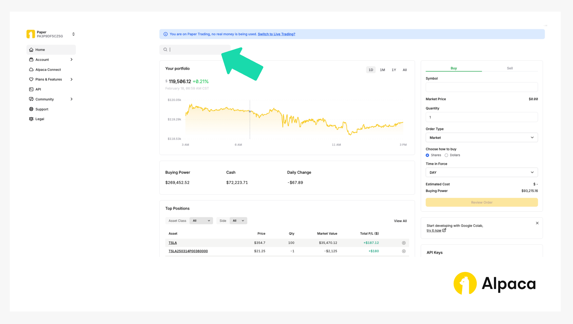
Sign in to your account and navigate to the “Home” page.

Step 2. Find your desired trade

On your dashboard in the top left, we can select between using your paper trading or live accounts. It’s important that we select the appropriate trading account before implementing an options strategy. If we want to practice without the risk of real capital, we can use your paper trading accounts. If we are looking to implement strategies, we can use your live account.

Once you’ve selected the desired account within your dashboard, we can monitor your portfolio, access market data, execute trades, and review your trading history. In order to create your first options trade, use the search bar to find and select the applicable option ticker symbol.

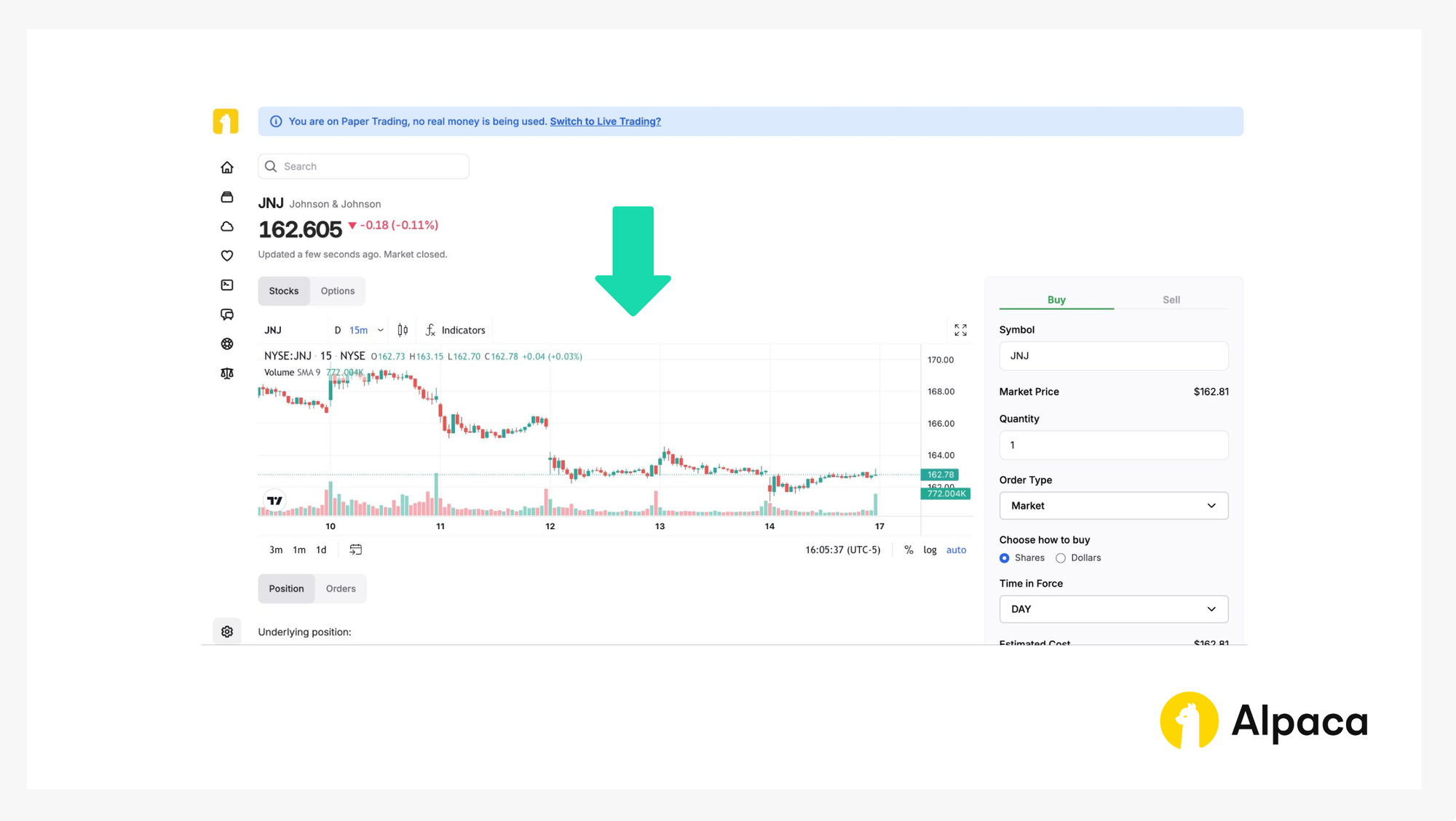
Step 3. Check underlying security’s bar chart

If we search the desired underlying asset, a page shows the asset’s bar chart. We can use this bar chart for a simple analysis.

Step 4. Opening an options position

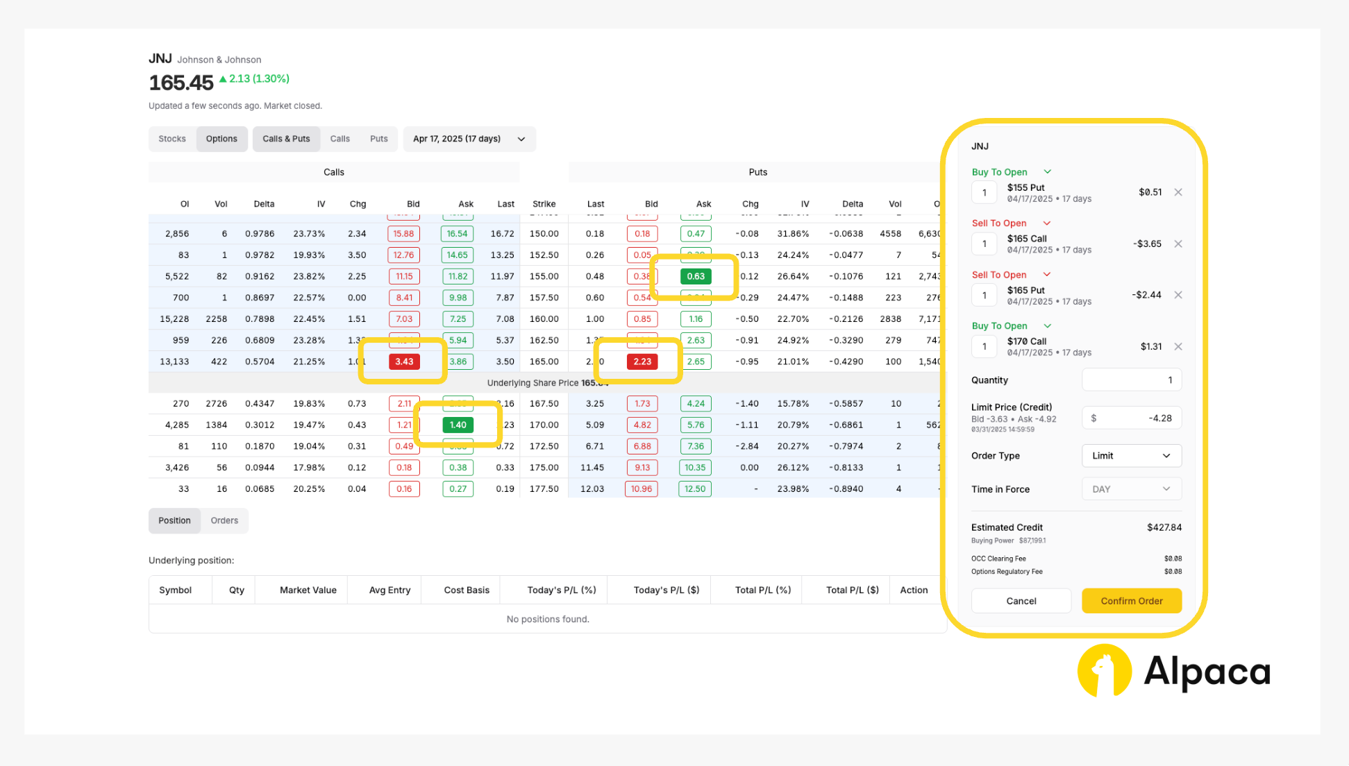
Assume we have already analyzed the market and determined the strike price for the four legs as follows: long put option to be $155.00; short put to be $165.00; short call to be $165.00; and long call to be $170 at the expiration date of April 17, 2025. Once determined, select and review your order type (market or limit) and decide on the number of contracts you’d like to trade. We can select up to four legs for the level 3 option trading at Alpaca. 

On the asset’s page, toggle from “Stocks” to “Options” and determine your desired contract type between calls and puts. We can also adjust the expiration date from the dropdown, ranging anywhere from 0DTE options to contracts hundreds of days in the future.

A short iron butterfly, for example, requires longing OTM put options, shorting ATM put options, shorting ATM call options, and longing OTM call options. Therefore, we can establish your position in the dashboard by selecting one long put option with "Buy To Open,” one short put option with “Sell To Open,” one short call option with “Sell To Open,” and one long call option with “Buy To Open” to purchase the options contracts.

Please note: The order in which we select the options does not matter. Additionally, on Alpaca’s dashboard and Trading API, credits are displayed as negative values, while debits appear as positive values. For example, in the image below, a credit spread (where your initial entry obtains premiums) is shown with a negative limit price (-$4.28 in this case) under 'Limit Price (Credit),' reflecting a total credit of $427.84 (with an extra 8 cents for the OCC Clearing Fee and Options Regulatory Fee).

Once selected, review your order type (such as market, limit, stop, stop limit, or trailing stop) and the number of contracts you’d like to trade. Click the “Confirm Order” button on the bottom right.

Your paper trading account will then mimic the execution of the order as though it were a real transaction.

Optional: Cancel your order

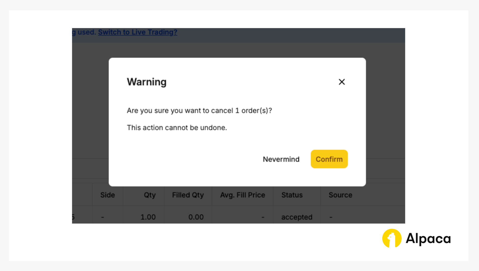
Keep in mind that with a multi-leg options order, we cannot cancel or replace an individual child leg. We can only cancel or replace the entire multi-leg options order. To do this, navigate to the 'Order' section, select the order we want to cancel, and click the 'Cancel 1 selected' button.

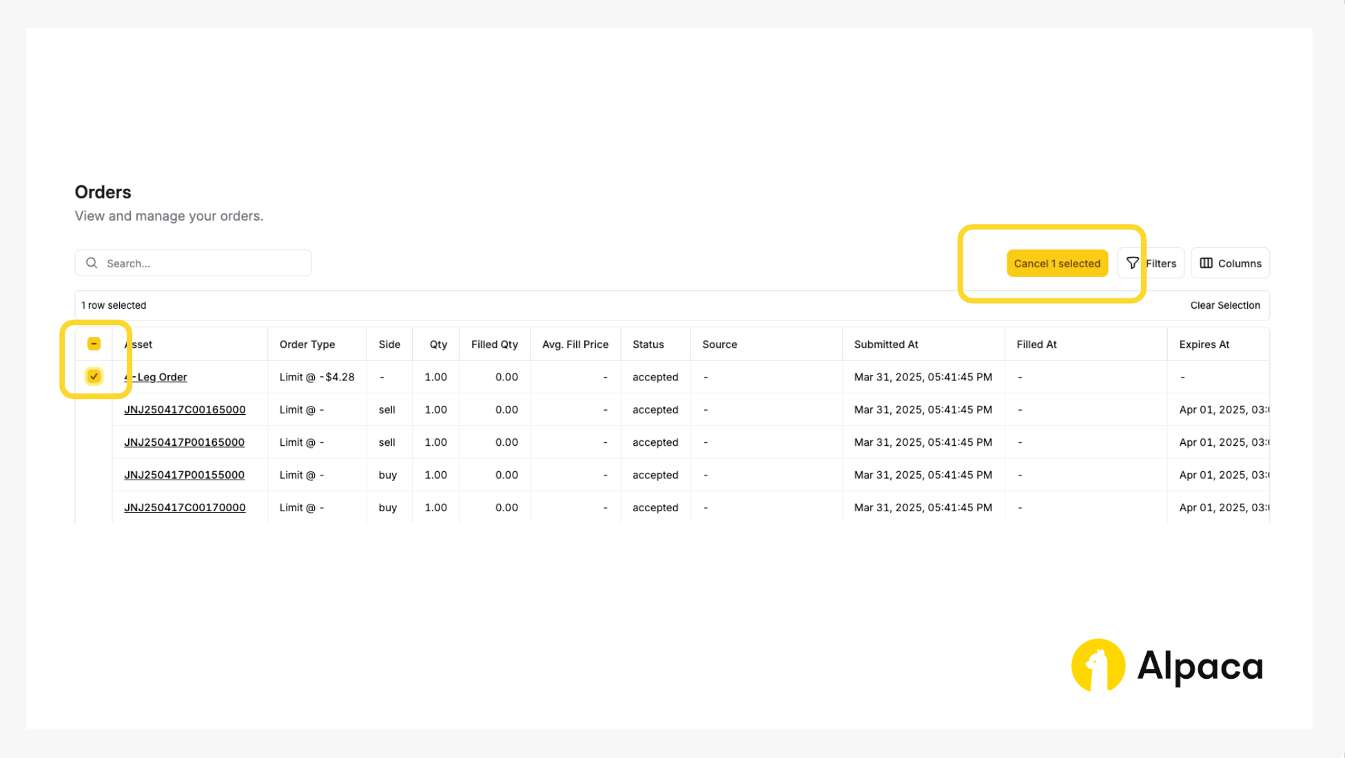
You’ll then be prompted to confirm.

Step 5. Closing your position

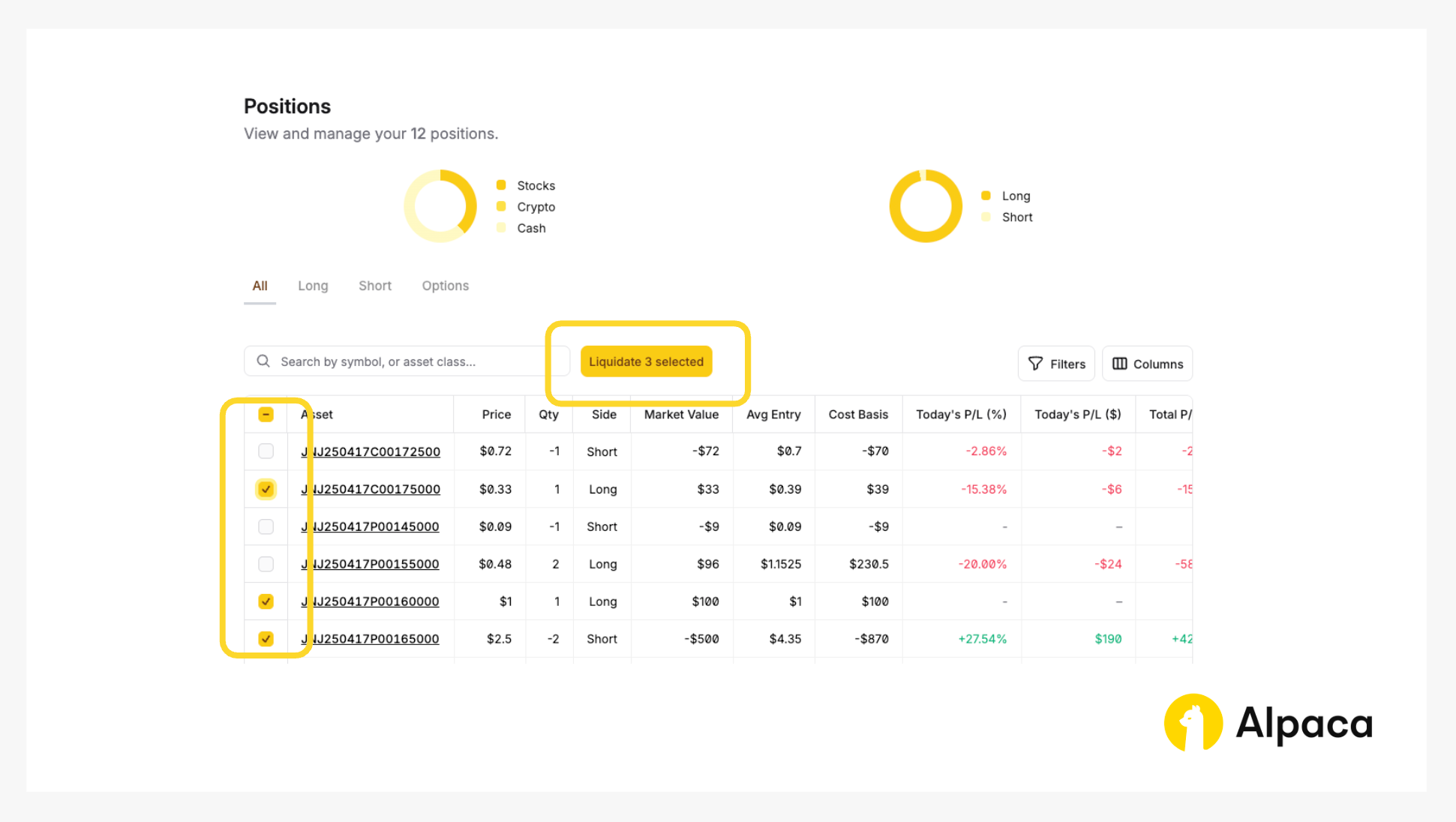
Closing an options position involves selling the options contract that we previously bought (in a long position) or buying back the options contract that we previously sold (in a short position). Either action terminates, or “closes”, your associated position.

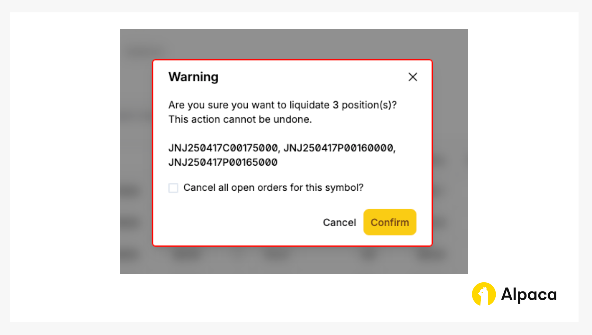
If you’d like to close your position, find the desired options contract on your “Home” page or under “Positions”. Click on the appropriate contract symbol and select “Liquidate 2 selected” to close your short iron butterfly position.

We will, then, click the “Confirm” button to liquidate the position.

Conclusion

The iron butterfly offers traders a defined-risk approach centered around a single core strike price. Constructed by combining vertical put and call spreads that share this central short strike, it provides distinct variations—long and short—allowing traders to structure positions based on their volatility outlook and market forecast, while clearly defining potential profits and losses from the outset.

Effective risk management is very important when implementing any iron butterfly variation. Traders should thoroughly assess market conditions, particularly volatility expectations (which dictates whether a long or short butterfly might be considered), select appropriate wing widths to manage maximum risk, and continuously monitor positions to make informed adjustments as needed. It's important to recognize that, like all trading strategies, the iron butterfly does not guarantee profits and carries inherent risks.

Continuous learning and diligent research are highly beneficial for mastering the nuances of both long and short iron butterfly strategies and understanding when market conditions might favor one over the other. Utilizing tools such as Alpaca's paper trading platform can provide valuable hands-on experience in managing these positions without financial exposure.

We hope you've found this guide on the iron butterfly insightful and useful for exploring this strategy further. As you put these concepts into practice, feel free to share your feedback and experiences on our forum, Slack community, or subreddit! And don't forget to check out the rest of our options-related tutorials.

For those looking to integrate options trading with Alpaca’s Trading API, here are some additional resources:

• Sign up for an Alpaca Trading API account
• How to Connect to Alpaca's Trading API
• How to Start Paper Trading with Alpaca's Trading API
• How to Trade Options with Alpaca’s Trading API
• Learn more credit spreads
• Read more Options Trading Tutorials
• Documentation: Options Trading

Execute your trading algos commission-free

Sign Up for Free

FAQs

What is an example of an iron butterfly option?

An iron butterfly option strategy has both a long and short version. In a short iron butterfly, a trader might sell an at-the-money call and an at-the-money put while buying an out-of-the-money call and put to cap potential losses; for example, if an underlying asset is trading at $100, selling both options at $100 while purchasing a $105 call and a $95 put creates a classic short iron butterfly that earns a net credit. Conversely, a long iron butterfly reverses these positions—the trader buys the at-the-money call and put and sells the out-of-the-money call and put—resulting in a net debit trade designed to profit when the asset makes a significant move away from current strike price.

Is an iron butterfly a good strategy?

The effectiveness of an iron butterfly strategy largely depends on market conditions and the trader’s outlook. The short iron butterfly strategy may be used when markets where the underlying asset remains close to the at-the-money strike, offering defined risk and an upfront credit; however, it suffers if the asset experiences unexpected, sharp price movements. In contrast, the long iron butterfly is designed for volatile environments—it may profit from significant moves in either direction but requires the anticipated volatility to materialize in order to overcome the cost of the net debit.

What is the difference between options butterfly and iron butterfly?

The key difference lies in their construction and inherent risk profiles. An options butterfly typically employs only calls or only puts by combining the purchase and sale of options to establish a limited risk/reward position that benefits when the underlying remains near the middle strike. An iron butterfly, however, uses both calls and puts by selling an at-the-money straddle and hedging with out-of-the-money options; it can be structured as either a net credit (short iron butterfly) or a net debit (long iron butterfly), resulting in distinct payoff dynamics and exposure to market volatility.

Which is better: iron condor or iron butterfly?

Determining whether an iron condor or an iron butterfly is better depends on your market expectations and risk tolerance. An iron condor provides a wider range of profitability through two vertical spreads, making it ideal for moderately stable markets where the underlying trades within a broader range. In contrast, an iron butterfly—particularly the short variant—theoretically offers maximum profit only if the asset finishes exactly at the central strike, while the long variant profits from significant price movement. Ultimately, the optimal choice hinges on whether you anticipate a relatively stable market or expect substantial volatility.

Options trading is not suitable for all investors due to its inherent high risk, which can potentially result in significant losses. Please read Characteristics and Risks of Standardized Options before investing in options.

Past hypothetical backtest results do not guarantee future returns, and actual results may vary from the analysis.

The Paper Trading API is offered by AlpacaDB, Inc. and does not require real money or permit a user to transact in real securities in the market. Providing use of the Paper Trading API is not an offer or solicitation to buy or sell securities, securities derivative or futures products of any kind, or any type of trading or investment advice, recommendation or strategy, given or in any manner endorsed by AlpacaDB, Inc. or any AlpacaDB, Inc. affiliate and the information made available through the Paper Trading API is not an offer or solicitation of any kind in any jurisdiction where AlpacaDB, Inc. or any AlpacaDB, Inc. affiliate (collectively, “Alpaca”) is not authorized to do business.

Please note that this article is for general informational purposes only and is believed to be accurate as of the posting date but may be subject to change. The examples above are for illustrative purposes only.

All investments involve risk, and the past performance of a security, or financial product does not guarantee future results or returns. There is no guarantee that any investment strategy will achieve its objectives. Please note that diversification does not ensure a profit, or protect against loss. There is always the potential of losing money when you invest in securities, or other financial products. Investors should consider their investment objectives and risks carefully before investing.

Securities brokerage services are provided by Alpaca Securities LLC ("Alpaca Securities"), member FINRA/SIPC, a wholly-owned subsidiary of AlpacaDB, Inc. Technology and services are offered by AlpacaDB, Inc.

This is not an offer, solicitation of an offer, or advice to buy or sell securities or open a brokerage account in any jurisdiction where Alpaca Securities are not registered or licensed, as applicable.