The Bear Put Spread Explained (and How to Trade The Options Strategy with Alpaca)
A bear put spread is an options strategy designed for traders anticipating a moderate decline in the price of an underlying asset. In this tutorial, we will explore the fundamentals of a bear put spread, providing real-world examples and discussing how market factors, including the option Greeks, influence their performance. We will also explore the risks and nuances that every trader should understand before executing this strategy.
By breaking down the mechanics and construction of a bear put spread, this guide aims to equip readers with the knowledge needed to effectively implement this strategy. We will also highlight actionable steps you can take for algorithmic integration using Alpaca's Trading API or manual trading using Alpaca’s dashboard.
To get the most out of this guide, explore the following resources first:
What is a Bear Put Spread?
The bear put spread strategy, also known as a put debit spread, involves purchasing a put option at a higher strike price while simultaneously selling another put option at a lower strike price, both with the same expiration date and underlying asset. The goal is to capitalize on the asset's downward movement while limiting both potential gains and losses.
A bear put spread is an options strategy involving two legs:
- Buying (longing) one put option at a higher strike price (out-of-the-money: OTM).
- Selling (shorting) another put option at a lower strike price (further OTM).
This setup creates a defined-risk, defined-reward position, often used by traders who expect the underlying price to decline modestly—but not necessarily plummet.
When to Use the Bear Put Spread Strategy
The bear put spread is designed for traders who anticipate a moderate decline in the price of the underlying asset. This makes it particularly useful in market environments where there is some pessimism about price depreciation, but not the expectation of a significant downward move. Compared to buying a single put option, this spread reduces the upfront cost by selling a lower-strike put, which helps offset the cost of the higher-strike long put.
The following market conditions may be when to utilize a bear put spread:
- Moderate bearish outlook: The trader expects the underlying asset to decrease modestly over the life of the options, but not necessarily plunge to significantly lower levels.
- Stable volatility: When implied volatility (IV) is relatively stable, the premiums for both puts are less inflated, making it easier to enter the spread at a reasonable net debit.
On the other hand, there are certain situations where a bear put spread may not be the ideal choice:
- Highly bearish expectations: If you expect a sharp and substantial decrease in the underlying price, buying a standalone long put may be a better fit. The capped profit potential of the bear put spread would limit gains in a fast-declining market.
- Bullish or uncertain outlook: If the trader believes the price will remain flat or rise, a bear put spread would likely lose its entire premium, since both puts would expire worthless.
- Narrow price movement (low volatility risk): If the underlying asset’s price barely moves, neither put option will gain much value, and the trader risks losing the net debit paid.
- Short-term time decay (Theta risk): Like any options strategy, the passage of time works against the bear put spread. If the underlying price doesn’t move favorably, the options’ time value will gradually decay, which can erode the spread’s value before expiration.
How to Build a Bear Put Spread Strategy
To construct a bear put spread, follow these steps:
- Select the underlying asset: Choose a stock or other asset that you expect to decline moderately in price.
- Determine the expiration date: Decide on the time frame in which you anticipate the price decline to occur.
- Choose the strike prices: Select two strike prices—one higher and one lower. The higher strike price will be for the long put, and the lower strike price will be for the short put.
- Enter the trade: Simultaneously buy the higher-strike put option and sell the lower-strike put option with the same expiration date.
Bear Put Spread Example (With Payoff Diagram)
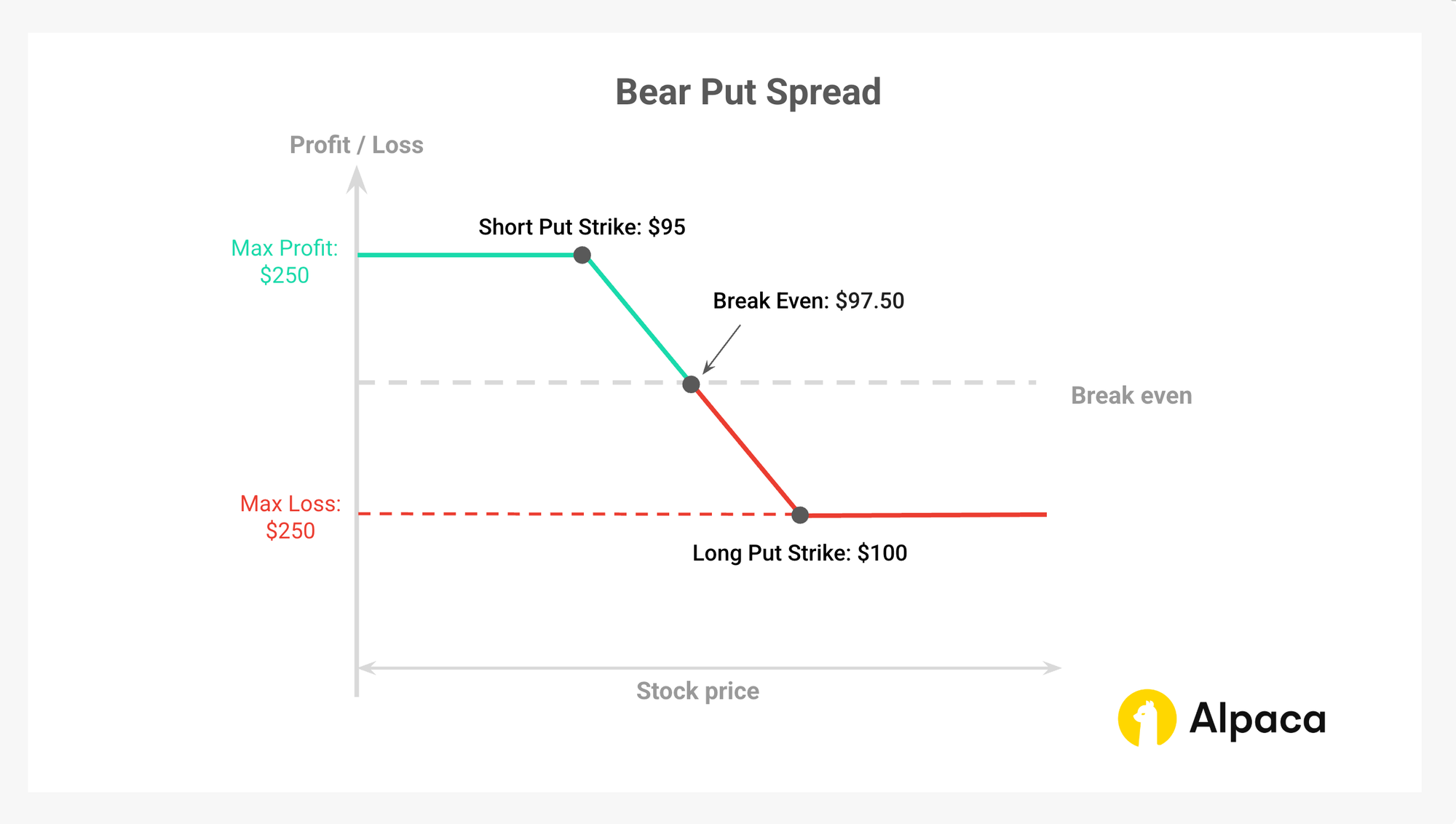
To understand how a bear put spread performs under various market conditions, let's analyze an example using stock XYZ as the underlying asset. This will help illustrate the risk-reward profile of a bear put spread, where the theoretical maximum loss is limited to the initial net debit, and the profit potential is theoretically limited to the difference between the strike prices minus the net debit.
Example Setup:
- Stock price at initiation: XYZ is trading at $100
- Strike Prices: Long put at $100, short put at $95
- Premiums:
- Long put (strike $100): $6.00 ($600 total)
- Short put (strike $95): $3.50 ($250 total)
- Net Debit (Total Cost): $3.50 - $6.00 = -$2.50 (-$250 total)
- Break Even Point: $100 (long put strike) - $2.50 (initial debit) = $97.50
Trade Structure:
Potential Outcomes at Expiration:
Scenario 1: Stock remains at $100 (at the long put strike) or rises
- If XYZ’s stock price stays at $100 or rises at expiration, both put options expire worthless. The long put (strike $100) finishes at-the-money (ATM), and the short put (strike $95) also expires worthless.
- The trader loses the entire net debit of $2.50 per share ($250 total for one spread).
- Net loss: $0 (both puts expire) - $250 (initial debit) = −$250 (theoretical maximum loss)
Scenario 2: Stock falls to $97.50 (break even point)
- At $97.50, the long put option (strike $100) has $2.50 of intrinsic value, while the short put (strike $95) is still OTM and expires worthless. This $2.50 of intrinsic value exactly offsets the initial $2.50 net debit paid to enter the spread.
- The trader breaks even at this price.
- Net even: $10,000 (exercising long put) - $9,750 (buying at the market price) - $250 (initial debit) = $0 (break-even)
Scenario 3: Stock falls to $92 (below both strikes)
- At $92, the long put (strike $100) has $8 or more of intrinsic value, and the short put (strike $95) is also in-the-money (ITM) with $3 of intrinsic value. The spread reaches its theoretical maximum value of $5 (the difference between the strike prices).
- The trader’s net profit is $2.50 per share ($250 total for one spread) after subtracting the initial $2.50 debit.
- Net profit: $10,000 (exercising long put) - $9,500 (being assigned short put) - $250 (initial debit) = $250 (theoretical maximum profit)
Key Metrics:
- Theoretical Maximum Loss: The net debit paid to enter the spread ($2.50 per share or $250 total).
- Theoretical Maximum Profit: The difference between the strike prices minus the net debit: ($5.00 - $2.50) = $2.50 per share ($250 total).
Note: For American-style options, there's a possibility of early assignment of the short call, especially around ex-dividend dates. This can affect the strategy's outcome before the expiration date.
Bear Call Spread vs. Bear Put Spread
Both bear call spreads and bear put spreads are similar in that both aim to profit from bearish market, but they differ in construction, cost, and risk profiles.
How the Greeks Factor into Bear Put Spreads
To optimize strategy execution when using a bear put spread, it is essential to monitor volatility trends, price movements, and expiration timelines, as various option Greek factors can influence the outcome.
Delta
- The bear put spread has a net negative delta, meaning it gains value as the stock price falls.
- Net delta is calculated by subtracting the short put’s delta from the long put’s delta.
- Unlike a single long put, a bear put spread’s delta remains relatively stable due to its low gamma.
- The impact of delta depends on the stock price’s position relative to the strike prices:
- Near the long put’s strike price: The net delta is moderately negative.
- Between the strikes: The net delta is most negative.
- Near the short put’s strike price: The net delta approaches zero or can be negative.
Gamma
- Compared to a single long put, the spread’s gamma is lower, reducing the extent of delta fluctuations.
- Net gamma is calculated by subtracting the short put’s gamma from the long put’s gamma.
- The impact of gamma depends on the stock price’s position relative to the strike prices:
- Near the long put’s strike price: The net gamma is positive.
- Between the strikes: The net gamma remains positive but diminishes.
- Near the short put’s strike price: The net gamma can become negative.
Theta
- As a debit strategy, time decay generally works against the bear put spread position (since you pay a net premium to enter the trade).
- The impact of theta depends on the stock price’s position relative to the strike prices:
- Near the long put’s strike price: The net theta is negative.
- Between the strikes: The net theta can be negative.
- Near the short put’s strike price: The net theta is positive.
Vega
- The vega of a bear put spread is lower compared to a single long put—due to the offsetting effects of the long and short puts, but vega is not uniformly low in all scenarios.
- The impact of vega depends on the stock price’s position relative to the strike prices:
- Near the long put’s strike price: The net vega is positive.
- Between the strikes: The net vega may remain positive.
- Near the short put’s strike price: The net vega is negative.
The Advantages and Disadvantages of Bear Put Spreads
Like any options strategy, the bear put spread has both benefits and limitations. Below is a breakdown of its key advantages and potential risks.
Advantages:
- Lower Cost Compared to Buying a Put: Selling the lower-strike put offsets part of the cost of buying the higher-strike put, reducing the initial investment.
- Defined Risk and Reward: Both potential losses and gains are limited and known upfront, aiding in precise risk management.
- Profit Potential in Moderately Bearish Markets: Suitable for scenarios where a trader expects a modest decline in the underlying asset's price.
- Partial Hedge Against Time Decay: The premium received from the short put helps offset the time decay of the long put.
Disadvantages and Risks:
- Capped Profit Potential: The theoretical maximum profit is limited to the difference between the strike prices minus the net debit, even if the underlying asset's price falls significantly.
- Time Decay Risk: If the underlying asset's price remains flat, the spread loses value over time due to theta decay.
- Sensitivity to Implied Volatility Changes: Decreasing IV can reduce the value of the spread, as the long put benefits more from higher IV than the short put.
- Possibility of Early Assignment: For American-style options, there's a risk of early assignment on the short put, especially if it becomes deep ITM.
- Liquidity Risk: Wide bid-ask spreads can impact execution quality, making it more challenging to enter or exit positions at desired prices.
- Directional Risk: The strategy requires the underlying asset's price to decline within a certain range; if the price increases or doesn't move as expected, the position can incur losses.

Building a Bear Put Spread Strategy With Alpaca’s Trading API
This section provides a step-by-step guide to implementing a bear put spread using Python and Alpaca’s Trading API in the Paper Trading environment. The strategy is a two-legged, directional strategy that involves simultaneously buying long put and short put options. This approach helps manage risk and optimize decision-making by leveraging key metrics and filters.
To get the most out of this guide, explore the following resources first:
Important Notes:
- The code assumes a flat interest rate, excludes dividends, and is not optimized for 0DTE options. It does not consider market hours and serves as a starting point rather than a complete strategy.
- Expiration Day Order Rules:
- Orders must be submitted before 3:15 p.m. ET for stocks/options and 3:30 p.m. ET for broad-based ETFs (e.g., SPY, QQQ).
- Orders placed after these times will be rejected.
- Expiring positions are auto-liquidated at 3:30 p.m. ET (stocks/options) and 3:45 p.m. ET (broad-based ETFs) for risk management.
- Multi-Leg (MLeg) Orders:
- All legs of a strategy must be included in the same order for acceptance.
- This is crucial for strategies with uncovered short options (e.g., short put calendar spreads, short call calendar spreads), which require Level 4 approval. See Alpaca's multi-leg order restrictions for details.
- American-Style Options Considerations:
- American-style options may be assigned early, affecting trade outcomes. Profit/loss scenarios assume expiration without early exercise and do not factor in transaction fees (e.g., brokerage fees, commissions). Traders should also monitor ex-dividend dates for short calls to manage assignment risk.
- Example equity:
- "AAPL" is used for demonstration purposes and should not be considered investment advice.
Step 1: Setting Up the Environment and Trade Parameters
The first step involves configuring the environment for trading a bear put spread and specifying your Alpaca Paper Trading API keys. This ensures your API connections and variable setup are secure and streamlined for data retrieval and trading operations.
Note: While we are using Jupyter Notebook for this tutorial, you can use Google Collab or any other IDE as your code environment. You can also find all of the below code on Alpaca’s Github page.
# Install or upgrade the package `alpaca-py` and import it
!python3 -m pip install --upgrade alpaca-py

import pandas as pd
import numpy as np
from scipy.stats import norm
import time
from scipy.optimize import brentq
from datetime import datetime, timedelta
from zoneinfo import ZoneInfo
from dotenv import load_dotenv
import os
from typing import Any, Dict, List, Optional, Tuple

import alpaca
from alpaca.data.timeframe import TimeFrame, TimeFrameUnit
from alpaca.data.historical.option import OptionHistoricalDataClient
from alpaca.data.historical.stock import StockHistoricalDataClient, StockLatestTradeRequest
from alpaca.data.requests import StockBarsRequest, OptionLatestQuoteRequest, OptionSnapshotRequest
from alpaca.trading.client import TradingClient
from alpaca.trading.requests import (
    MarketOrderRequest,
    GetOptionContractsRequest,
    MarketOrderRequest,
    OptionLegRequest,
    ClosePositionRequest,
)
from alpaca.trading.enums import (
    AssetStatus,
    OrderSide,
    OrderClass,
    OrderStatus,
    TimeInForce,
    ContractType,
)
The script initializes Alpaca clients for trading stocks and options, as well as for handling data requests.
# API credentials for Alpaca
API_KEY = "YOUR_ALPACA_API_KEY_FOR_PAPER_TRADING"
API_SECRET = 'YOUR_ALPACA_API_SECRET_KEY_FOR_PAPER_TRADING'
BASE_URL = None
## We use paper environment for this example (Please do not modify this. This example is for paper trading only)
PAPER = True

# Initialize Alpaca clients
trade_client = TradingClient(api_key=API_KEY, secret_key=API_SECRET, paper=PAPER, url_override=BASE_URL)
option_historical_data_client = OptionHistoricalDataClient(api_key=API_KEY, secret_key=API_SECRET, url_override=BASE_URL)
stock_data_client = StockHistoricalDataClient(api_key=API_KEY, secret_key=API_SECRET)

# Below are the variables for development this documents
# Please do not change these variables
trade_api_url = None
trade_api_wss = None
data_api_url = None
option_stream_data_wss = None
Step 2: Calculations for Implied Volatility and Option Greeks with Black-Scholes model
The calculate_implied_volatility function estimates implied volatility (IV) using the Black-Scholes model. The function defines a reasonable range for sigma (1e-6 to 5.0) to avoid extreme values. For deep OTM options where the price is close to intrinsic value, the function directly sets IV to 0.0 to prevent calculation errors. A numerical root-finding method is used to solve for IV, ensuring accuracy even in edge cases.
# Calculate implied volatility
def calculate_implied_volatility(option_price, S, K, T, r, option_type):

    # Define a reasonable range for sigma
    sigma_lower = 1e-6
    sigma_upper = 5.0  # Adjust upper limit if necessary

    # Check if the option is out-of-the-money and price is close to zero
    intrinsic_value = max(0, (S - K) if option_type == 'call' else (K - S))
    if option_price <= intrinsic_value + 1e-6:

        print('Option price is close to intrinsic value; implied volatility is near zero.')
        return 0.0

    # Define the function to find the root
    def option_price_diff(sigma):
        d1 = (np.log(S / K) + (r + 0.5 * sigma ** 2) * T) / (sigma * np.sqrt(T))
        d2 = d1 - sigma * np.sqrt(T)
        if option_type == 'call':
            price = S * norm.cdf(d1) - K * np.exp(-r * T) * norm.cdf(d2)
        elif option_type == 'put':
            price = K * np.exp(-r * T) * norm.cdf(-d2) - S * norm.cdf(-d1)
        return price - option_price

    try:
        return brentq(option_price_diff, sigma_lower, sigma_upper)
    except ValueError as e:
        print(f"Failed to find implied volatility: {e}")
        return None
The calculate_greeks function estimates all option Greeks: delta, gamma, theta, and vega based on the implied volatility calculated through calculate_implied_volatility. In this demonstration, we mainly use delta and implied volatility.
def calculate_greeks(option_price, strike_price, expiration, underlying_price, risk_free_rate, option_type):
    T = (expiration - pd.Timestamp.now()).days / 365 # It is unconventional, but some use 225 days (# of annual trading days) in replace of 365 days
    T = max(T, 1e-6)  # Set minimum T to avoid zero

    if T == 1e-6:
        print('Option has expired or is expiring now; setting Greeks based on intrinsic value.')
        if option_type == 'put':
            delta = -1.0 if underlying_price < strike_price else 0.0
        else:
            delta = 1.0 if underlying_price > strike_price else 0.0
        gamma = 0.0
        theta = 0.0
        vega = 0.0
        return delta, gamma, theta, vega

    # Calculate IV
    IV = calculate_implied_volatility(option_price, underlying_price, strike_price, T, risk_free_rate, option_type)

    if IV is None or IV == 0.0:
        print('Implied volatility could not be determined, skipping Greek calculations.')
        return None

    d1 = (np.log(underlying_price / strike_price) + (risk_free_rate + 0.5 * IV ** 2) * T) / (IV * np.sqrt(T))
    d2 = d1 - IV * np.sqrt(T) # d2 for Theta calculation
    # Calculate Delta
    delta = norm.cdf(d1) if option_type == 'call' else -norm.cdf(-d1)
    # Calculate Gamma
    gamma = norm.pdf(d1) / (underlying_price * IV * np.sqrt(T))
    # Calculate Vega
    vega = underlying_price * np.sqrt(T) * norm.pdf(d1) / 100
    # Calculate Theta
    if option_type == 'call':
        theta = (
            - (underlying_price * norm.pdf(d1) * IV) / (2 * np.sqrt(T))
            - (risk_free_rate * strike_price * np.exp(-risk_free_rate * T) * norm.cdf(d2))
        )
    else:
        theta = (
            - (underlying_price * norm.pdf(d1) * IV) / (2 * np.sqrt(T))
            + (risk_free_rate * strike_price * np.exp(-risk_free_rate * T) * norm.cdf(-d2))
        )
    # Convert annualized theta to daily theta
    theta /= 365

    return delta, gamma, theta, vega
Step 3: Pick Your Strategy Inputs
Underlying Price and Strike Range
The script retrieves the current AAPL price via Alpaca’s market data, then calculates the minimum and maximum strike prices by multiplying that price by (1 - 0.06) and (1 + 0.06), respectively. This ensures that the strike range covers ±5% around the market price.
Expiration Dates
The code sets a minimum (today + 21 days) and maximum (today + 60 days) for potential expirations. However, we further refine it to a common range of 21 to 60 days. This means the final options that are picked for the long put and short put must fall within that 21–60 day window, which is a common range for short to medium-term directional strategies or event-driven trades.
Additionally, the script incorporates a risk-free rate of 1% (0.01) in internal calculations, enhancing the accuracy of implied volatility and Greek metrics, particularly vega and gamma. This helps fine-tune pricing models and ensures a more precise evaluation of the straddle’s risk and reward dynamics.
Liquidity and Open Interest Threshold
To avoid thinly traded contracts, the code sets an Open Interest (OI) threshold of 50. This ensures that only options with sufficient liquidity are considered, leading to tighter spreads and smoother execution.
Option Greeks and IV Ranges
The criteria dictionary defines acceptable ranges for both legs of the bear put spread. For example, each option could have an expiration expiration between 21 and 60 days, an implied volatility (IV) between 0.20 and 0.50, a delta between -0.60 and -0.10 for the short put, and between -0.70 and -0.20 for the long put, and a vega between 0.01 and 0.20. These ranges help target options that are reasonably priced and not too deep ITM or OTM.
Target Profit
For the purposes of this example, we chose a target profit percentage of 40%, meaning the spread will be closed if the short_put’s value drops to 40% from the initial price. Additionally, stop-loss thresholds are set with a delta limit of -0.50 and a IV limit of 0.40, providing clear guidelines to exit the position if sensitivity to price or volatility moves beyond acceptable levels.
Buying Power Allocation
Only 5% of the account’s buying power (BUY_POWER_LIMIT = 0.05) is allocated to the trade. The code calculates the available buying power and ensures that the total cost of the spread remains within this conservative limit, helping maintain disciplined position sizing.
Evaluating the Risk
In order to calculate the theoretical maximum risk associated with a spread, we set buying_power_limit as a threshold to decide whether to enter the position or not. Traders can also set up alerts or automate exits when these thresholds are reached. Active monitoring or using limit orders is recommended to mitigate slippage in fast-moving markets.
Monitoring and Potential Adjustments
We set several thresholds for rolling or closing an entered position. In this example, these thresholds are applied to the short put options we sold to open the position.
The TARGET_PROFIT_PERCENTAGE is set to 0.4, meaning the spread will be closed if its value increases by 40% from the initial profit from the short put option. In addition, a DELTA_STOP_LOSS of 0.50 and an IV_STOP_LOSS of 0.40 are used to trigger an exit if the option’s delta or IV exceed these levels, helping manage risk during rapid price or volatility changes.
Traders can set up alerts or automate these exits to ensure positions are actively managed in fast-moving markets. Some traders may choose to monitor net delta or net IV for the entire spread rather than focusing solely on the short options. This choice depends on individual judgment and strategy.
Liquidity Considerations and Stop-Loss Limits
Because we set an open interest threshold (OI_THRESHOLD = 50), we’re already filtering out illiquid strikes. Still, be mindful that in a fast-moving market, option prices can gap, and a typical stop-loss order may trigger at less favorable prices. A common practice is often to monitor the position actively or use limit orders to exit, ensuring we don’t face excessive slippage.
# Select the underlying stock
underlying_symbol = 'AAPL'

# Set the timezone
timezone = ZoneInfo('America/New_York')

# Get current date in US/Eastern timezone
today = datetime.now(timezone).date()

# Define a 6% range around the underlying price
STRIKE_RANGE = 0.06

# Buying power percentage to use for the trade
BUY_POWER_LIMIT = 0.05

# Risk free rate for the options greeks and IV calculations
risk_free_rate = 0.01

# Check account buying power
buying_power = float(trade_client.get_account().buying_power)

# Set the open interest volume threshold
OI_THRESHOLD = 50

# Calculate the limit amount of buying power to use for the trade
buying_power_limit = buying_power * BUY_POWER_LIMIT

# Set the expiration date range for the options
min_expiration = today + timedelta(days=21)
max_expiration = today + timedelta(days=60)

# Get the latest price of the underlying stock
def get_underlying_price(symbol):
    # Get the latest trade for the underlying stock
    underlying_trade_request = StockLatestTradeRequest(symbol_or_symbols=symbol)
    underlying_trade_response = stock_data_client.get_stock_latest_trade(underlying_trade_request)
    return underlying_trade_response[symbol].price

# Get the latest price of the underlying stock
underlying_price = get_underlying_price(underlying_symbol)

# Set the minimum and maximum strike prices based on the underlying price
min_strike = str(underlying_price * (1 - STRIKE_RANGE))
max_strike = str(underlying_price * (1 + STRIKE_RANGE))

# Define the criteria for selecting the options
# Each key corresponds to a leg and maps to a tuple of: (expiration range, IV range, delta range, vega range)
criteria = {
    'short_put':  ((21, 60), (0.20, 0.50), (-0.60, -0.10), (0.01, 0.20)),
    'long_put': ((21, 60), (0.20, 0.50), (-0.70, -0.20), (0.01, 0.20))
}

# Set target profit levels
TARGET_PROFIT = 0.4
DELTA_STOP_LOSS = -0.50
IV_STOP_LOSS = 0.40

# Display the values
print(f"Underlying Symbol: {underlying_symbol}")
print(f"{underlying_symbol} price: {underlying_price}")
print(f"Strike Range: {STRIKE_RANGE}")
print(f"Buying Power Limit Percentage: {BUY_POWER_LIMIT}")
print(f"Risk Free Rate: {risk_free_rate}")
print(f"Account Buying Power: {buying_power}")
print(f"Buying Power Limit: {buying_power_limit}")
print(f"Open Interest Threshold: {OI_THRESHOLD}")
print(f"Minimum Expiration Date: {min_expiration}")
print(f"Maximum Expiration Date: {max_expiration}")
print(f"Minimum Strike Price: {min_strike}")
print(f"Maximum Strike Price: {max_strike}")
Step 4: Market Data Analysis with Underlying Assets
When implementing a bear put spread, it's essential to identify market conditions that support the strategy. Using a combination of price trends, volatility measures, and technical indicators, traders would be able to optimize entry points and improve trade efficiency. The following factors may help the bear put spread setups based on underlying asset price movement and volatility events.
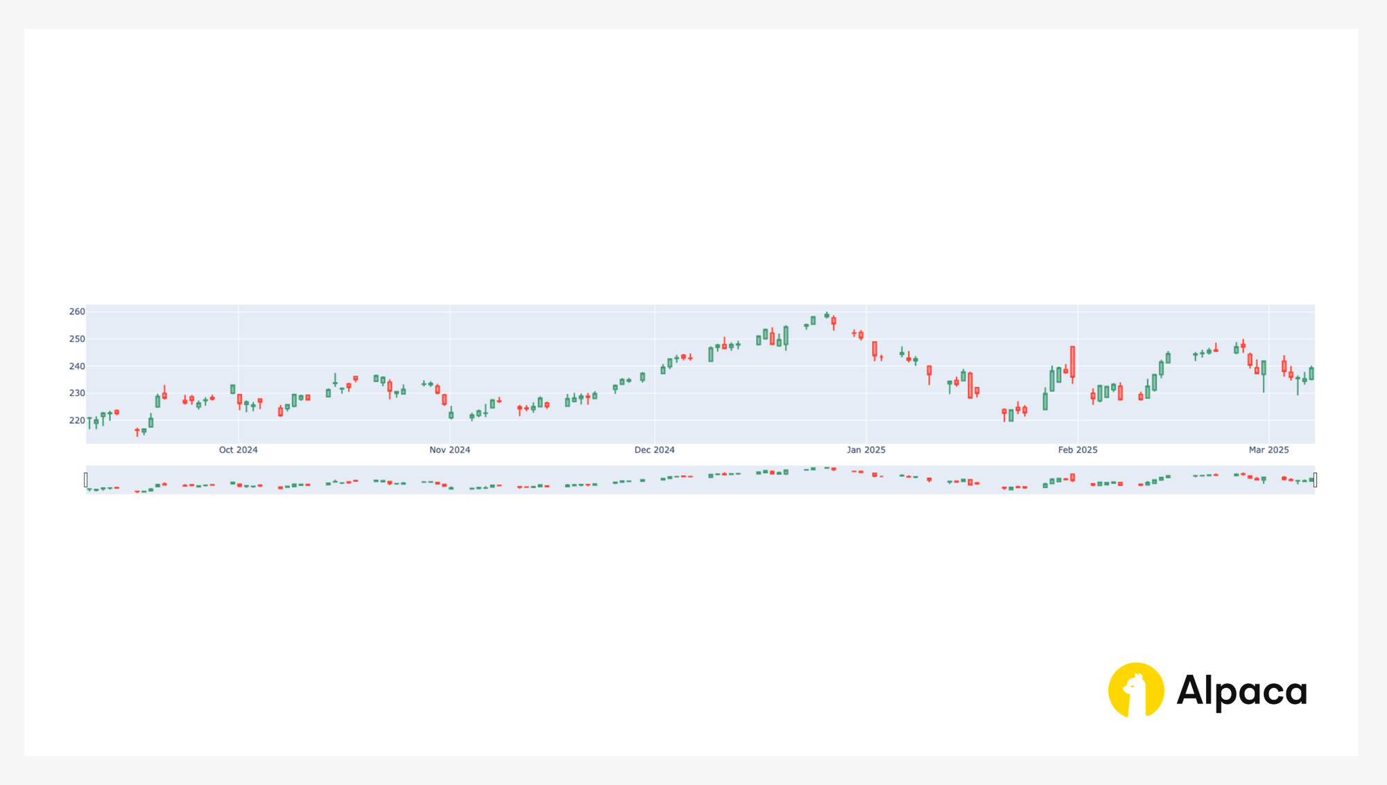
Stock Price Trends (Bar Chart Analysis)
Monitoring historical price movements can help traders evaluate the broader trend of the underlying asset before entering a bear put spread. Reviewing candlestick charts offers valuable insights into recent price action, as well as key support and resistance levels. This analysis may help traders identify whether the asset is trending upward or trading within a range.
A bear put spread works best in moderately bearish environments, where the price is expected to decrease gradually toward the short put’s strike price. It is less suitable for strongly bullish markets or highly volatile conditions, where sharp reversals could cause the spread to lose value before expiration.
# Get the historical data for the underlying stock by symbol and timeframe
# ref. https://alpaca.markets/sdks/python/api_reference/data/option/historical.html
def get_stock_data(underlying_symbol, days=90):
    today = datetime.now(timezone).date()
    req = StockBarsRequest(
        symbol_or_symbols=[underlying_symbol],
        timeframe=TimeFrame(amount=1, unit=TimeFrameUnit.Day),     # specify timeframe
        start=today - timedelta(days=days),                          # specify start datetime, default=the beginning of the current day.
    )
    return stock_data_client.get_stock_bars(req).df

# List of stock agg objects while dropping the symbol column
priceData = get_stock_data(underlying_symbol, days=180).reset_index(level='symbol', drop=True)

import plotly.graph_objects as go

# Bar chart for the stock price
fig = go.Figure(data=[go.Candlestick(x=priceData.index,
                open=priceData['open'],
                high=priceData['high'],
                low=priceData['low'],
                close=priceData['close'])])

fig.show()
This code returns the bar chart like in the image below.
Relative Volatility Index (RVI)
The Relative Volatility Index (RVI) measures the strength of price momentum relative to volatility. It helps confirm whether the market is experiencing increased price fluctuations or stabilizing.
If the RVI is between 40 and 60, it suggests moderately neutral volatility, which may be favorable as an entry point for a bear put spread strategy. Conversely, a low or declining RVI may indicate a stable market environment, making it a less favorable setup at the time of entry. However, since volatility contraction can either benefit or harm the strategy by accelerating premium decay in the options, it is important to actively monitor the RVI.
def calculate_rvi(df, period):
    # Calculate daily price changes
    df['price_change'] = df['close'].diff()

    # Separate up and down price changes
    df['up_change'] = df['price_change'].where(df['price_change'] > 0, 0)
    df['down_change'] = -df['price_change'].where(df['price_change'] < 0, 0)

    # Calculate std of up and down changes over the rolling period
    df['avg_up_std'] = df['up_change'].rolling(window=period).std()
    df['avg_down_std'] = df['down_change'].rolling(window=period).std()

    # Calculate RVI
    df['rvi'] = 100 - (100 / (1 + (df['avg_up_std'] / df['avg_down_std'])))

    # Smooth the RVI with a 4 periods moving average
    df['rvi_smoothed'] = df['rvi'].rolling(window=4).mean()

    return df['rvi_smoothed']

# smoothed RVI
calculate_rvi(priceData, period=21).iloc[30:]
Bollinger Bands for Volatility Assessment
Bollinger Bands provide a dynamic range around the asset's price, helping traders assess current market volatility and potential price extremes. When the underlying stock price approaches the upper Bollinger Band, it may indicate overbought conditions, while a move toward the lower band could suggest oversold levels.
For a bear put spread, Bollinger Bands can help identify whether the asset is in a favorable moderate downtrend, which is ideal for this strategy. A price trending downward toward the middle to lower band — without excessive volatility — may signal conditions where the stock could gradually move into the profitable zone between the long and short put strikes.
In contrast, if the asset is near the upper band or moving erratically, the chances of success for this strategy may decline, as sharp reversals or unpredictable price swings increase the risk of losing the initial premium paid for the spread.
# setup bollinger band calculations
def check_bb(df, period=14, multiplier=2):
    bollinger_bands = []
    # Calculate the Simple Moving Average (SMA)
    df['SMA'] = df['close'].rolling(window=period).mean()
    # Calculate the rolling standard deviation
    df['StdDev'] = df['close'].rolling(window=period).std()
    # Calculate the Upper Bollinger Band (two standard deviation)
    df['Upper Band'] = df['SMA'] + (multiplier * df['StdDev'])
    # Calculate the Lower Bollinger Band (two standard deviation)
    df['Lower Band'] = df['SMA'] - (multiplier * df['StdDev'])
    # Get the most recent Upper Band value
    upper_bollinger_band = df['Upper Band'].iloc[-1]
    lower_bollinger_band = df['Lower Band'].iloc[-1]

    bollinger_bands = [upper_bollinger_band, lower_bollinger_band]
    return bollinger_bands

bollinger_bands = check_bb(priceData, 14, 2)

# The current market price is not too close to the two-standard deviation level yet but is relatively closer to the higher Bollinger Band.
print(f"Latest Upper Bollinger Band is: {bollinger_bands[0]}. Latest Lower Bollinger Band is {bollinger_bands[1]}; while underlying stock '{underlying_symbol}' price is {underlying_price}.")
Step 5: Set up for A bear put spread (Find both short and long put options)
This code sets up a tool for printing messages from the code. It tells python to show general messages (INFO level) and more detailed messages (DEBUG level) so we can see what's happening and troubleshoot if needed.
# Configure logging
import logging
logging.basicConfig(level=logging.INFO)
logger = logging.getLogger(__name__)
logger.setLevel(logging.DEBUG)
The get_options function retrieves active option contracts for a specified underlying symbol within a given strike price and expiration date range. Reminder to specify option_type as either ContractType.CALL or ContractType.PUT to filter for the desired option type.
# option_type: ContractType.CALL or ContractType.PUT.
def get_options(underlying_symbol, min_strike, max_strike, min_expiration, max_expiration, option_type):
    req = GetOptionContractsRequest(
        underlying_symbols=[underlying_symbol],
        status=AssetStatus.ACTIVE,
        type=option_type,
        strike_price_gte=min_strike,
        strike_price_lte=max_strike,
        expiration_date_gte=min_expiration,
        expiration_date_lte=max_expiration,
    )
    return trade_client.get_option_contracts(req).option_contracts
The helper function validate_sufficient_OI verifies that an option's data includes the necessary fields and that its open interest exceeds a specified threshold. It is used at the start of the workflow to ensure that only eligible options are processed further.
def validate_sufficient_OI(option_data, OI_THRESHOLD):
    '''Ensure that the option has the required fields and sufficient open interest.'''
    if option_data.open_interest is None or option_data.open_interest_date is None:
        return False
    if float(option_data.open_interest) <= OI_THRESHOLD:
        return False
    return True
The calculate_option_metrics function calculates key metrics for an option contract. It starts by retrieving the latest quote for the option (using the option’s symbol) and computes the mid-price from the bid and ask prices. Then, it determines the option’s expiration date and the number of days remaining until expiration. Using these values, it calculates the implied volatility and the Greeks (delta, gamma, theta, and vega) by calling helper functions. Finally, it returns all these computed metrics as a dictionary for later use.
def calculate_option_metrics(option_data, underlying_price, risk_free_rate):
    """
    Calculate key option metrics including option price, implied volatility (IV), and option Greeks.
    """
    # Retrieve the latest quote for the option
    option_quote_req = OptionLatestQuoteRequest(symbol_or_symbols=option_data['symbol'])
    option_quote = option_historical_data_client.get_option_latest_quote(option_quote_req)[option_data['symbol']]
    option_price = (option_quote.bid_price + option_quote.ask_price) / 2

    # Calculate expiration and remaining days
    expiration_date = pd.Timestamp(option_data['expiration_date'])
    remaining_days = (expiration_date - pd.Timestamp.now()).days

    # Calculate implied volatility
    iv = calculate_implied_volatility(
        option_price=option_price,
        S=underlying_price,
        K=float(option_data['strike_price']),
        T=max(remaining_days / 365, 1e-6),
        r=risk_free_rate,
        option_type=option_data['type'].value
    )

    # Calculate Greeks (delta and vega)
    delta, gamma, theta, vega = calculate_greeks(
        option_price=option_price,
        strike_price=float(option_data['strike_price']),
        expiration=expiration_date,
        underlying_price=underlying_price,
        risk_free_rate=risk_free_rate,
        option_type=option_data['type'].value
    )

    return {
        'option_price': option_price,
        'expiration_date': expiration_date,
        'remaining_days': remaining_days,
        'iv': iv,
        'delta': delta,
        'gamma': gamma,
        'theta': theta,
        'vega': vega
    }
This function ensures that the provided option_data is in dictionary format. If option_data is given in a different format (e.g. OptionContract object), it converts it to a dictionary.
def ensure_dict(option_data):
    """
    Convert option_data to a dict using model_dump() if available (for Pydantic models),
    otherwise return the data as-is.
    """
    if hasattr(option_data, "model_dump"):
        return option_data.model_dump()
    return option_data
The build_option_dict function builds a comprehensive option dictionary by merging the raw option data with the calculated metrics from calculate_option_metrics. It first converts the input to a dictionary using ensure_dict, then obtains all necessary metrics (like option price, IV, delta, and vega). Finally, it constructs and returns a candidate dictionary that includes both the original option details (such as id, name, symbol, strike price, etc.) and the calculated metrics. This consolidated dictionary can be used for further processing or trading decisions.
def build_option_dict(option_data, underlying_price, risk_free_rate):
    """
    Build an option dictionary by merging raw option data with calculated metrics.
    """
    option_data = ensure_dict(option_data)  # Convert to dict if necessary
    metrics = calculate_option_metrics(option_data, underlying_price, risk_free_rate)
    candidate = {
        'id': option_data['id'],
        'name': option_data['name'],
        'symbol': option_data['symbol'],
        'strike_price': option_data['strike_price'],
        'root_symbol': option_data['root_symbol'],
        'underlying_symbol': option_data['underlying_symbol'],
        'underlying_asset_id': option_data['underlying_asset_id'],
        'close_price': option_data['close_price'],
        'close_price_date': option_data['close_price_date'],
        'expiration_date': metrics['expiration_date'],
        'remaining_days': metrics['remaining_days'],
        'open_interest': option_data['open_interest'],
        'open_interest_date': option_data['open_interest_date'],
        'size': option_data['size'],
        'status': option_data['status'],
        'style': option_data['style'],
        'tradable': option_data['tradable'],
        'type': option_data['type'],
        'initial_IV': metrics['iv'],
        'initial_delta': metrics['delta'],
        'initial_gamma': metrics['gamma'],
        'initila_theta': metrics['theta'],
        'initial_vega': metrics['vega'],
        'initial_option_price': metrics['option_price'],
    }

    return candidate
The function check_candidate_option_conditions checks if a candidate option meets the filtering criteria provided as a tuple (expiration range, IV range, delta range, vega range). It is used within the main workflow to determine whether a candidate qualifies for a specific leg of the bear put spread.
def check_candidate_option_conditions(candidate, criteria, label):
    """
    Check whether a candidate option meets the filtering criteria.
    The criteria is a tuple of (expiration_range, iv_range, delta_range, vega_range).
    Logs detailed information if a candidate fails a criterion.
    """
    expiration_range, iv_range, delta_range, vega_range = criteria

    if not (expiration_range[0] <= candidate['remaining_days'] <= expiration_range[1]):
        logger.debug(f"{candidate['symbol']} fails expiration condition for {label}: remaining_days {candidate['remaining_days']} not in {expiration_range}.")
        return False
    if not (iv_range[0] <= candidate['initial_IV'] <= iv_range[1]):
        logger.debug(f"{candidate['symbol']} fails IV condition for {label}: initial_IV {candidate['initial_IV']} not in {iv_range}.")
        return False
    if not (delta_range[0] <= candidate['initial_delta'] <= delta_range[1]):
        logger.debug(f"{candidate['symbol']} fails delta condition for {label}: initial_delta {candidate['initial_delta']} not in {delta_range}.")
        return False
    if not (vega_range[0] <= candidate['initial_vega'] <= vega_range[1]):
        logger.debug(f"{candidate['symbol']} fails vega condition for {label}: initial_vega {candidate['initial_vega']} not in {vega_range}.")
        return False

    return True
The pair_put_candidates function identifies a valid bear put spread by pairing a long put and short put with the same expiration date. It ensures the short put’s strike is below the underlying price and the long call’s strike is above it, matching the typical setup for this strategy. The first matching pair is returned, or None if no valid pair is found.
def pair_put_candidates(short_puts, long_puts, underlying_price) -> Tuple[Optional[Dict[str, Any]], Optional[Dict[str, Any]]]:
    """
    For the bear put spread, require: short_put strike <= underlying_price < long_put strike.
    Returns the first valid pair found.
    """
    for sp in short_puts:
        for lp in long_puts:
            if sp['expiration_date'] == lp['expiration_date'] and sp['strike_price'] <= underlying_price < lp['strike_price']:
                logger.info(f"Selected Bear Put spread: short_put {sp['symbol']} and long_put {lp['symbol']} with expiration {sp['expiration_date']}.")
                return sp, lp


    # If no valid pair is found, log the expiration date (if available) from the candidate lists.
    expiration_info = None
    if short_puts:
        expiration_info = short_puts[0]['expiration_date']
    elif long_puts:
        expiration_info = long_puts[0]['expiration_date']

    if expiration_info:
        logger.info(f"No valid bear put spread pair found for expiration {expiration_info} with the given candidates and underlying price conditions.")
    else:
        logger.info("No valid bear put spread pair found: no candidate data available.")

    return [], []
This check_buying_power function calculates the net cost (risk) of entering a bear put spread and ensures it does not exceed the buying power limit. It compares the difference between the long put’s price and the short put’s price, multiplied by the contract size. If the cost is too high, it raises an exception to prevent the trade.
def check_buying_power(short_put, long_put, buying_power_limit):
    """
    Calculates the total premium paid (risk) for a bear put spread and checks it against the buying power limit.
    If the buying power requirement is not met, the exception is thrown and the rest of the code is never executed.
    """
    option_size = float(short_put['size'])
    risk = (long_put['initial_option_price'] - short_put['initial_option_price']) * option_size
    logger.info(f"Calculated bear put spread risk: {risk}.")

    if risk >= buying_power_limit:
        raise Exception('Buying power limit exceeded for a bear put spread risk.')
The find_options_for_bearl_put_spread function coordinates the process of finding and validating a bear put spread. It filters bear options based on criteria, groups potential long and short candidates by expiration, and attempts to pair them into valid spreads. If a suitable pair is found, it checks the spread’s buying power requirement before returning the first valid pair. If no valid spread is found, it returns an empty list.
def find_options_for_bear_put_spread(put_options, underlying_price, risk_free_rate, buying_power_limit, criteria, OI_THRESHOLD):
    """
    Orchestrates the workflow to build a bear put spread.
    Groups options by expiration, filters them with criteria, pairs candidates using helper functions,
    and checks buying power.

    Returns:
        A list of legs [short_put, long_put] if a valid pair is found, or an empty list otherwise.
    """
    short_put_candidates_by_exp: Dict[pd.Timestamp, List[Dict[str, Any]]] = {}
    long_put_candidates_by_exp: Dict[pd.Timestamp, List[Dict[str, Any]]] = {}

    # Process each option candidate
    for option_data in put_options:
        if not validate_sufficient_OI(option_data, OI_THRESHOLD):
            logger.warning(f"Insufficient open interest for option {getattr(option_data, 'symbol', 'unknown')} (threshold: {OI_THRESHOLD}). Skipping candidate.")
            continue

        candidate = build_option_dict(option_data, underlying_price, risk_free_rate)
        expiration_date = candidate['expiration_date']
        short_put_candidates_by_exp.setdefault(expiration_date, [])
        long_put_candidates_by_exp.setdefault(expiration_date, [])

        # Check each candidate for both put criteria
        if check_candidate_option_conditions(candidate, criteria['short_put'], 'short_put'):
            short_put_candidates_by_exp[expiration_date].append(candidate)
            logger.info(f"Added {candidate['symbol']} as a short put candidate for expiration {expiration_date}.")
        if check_candidate_option_conditions(candidate, criteria['long_put'], 'long_put'):
            long_put_candidates_by_exp[expiration_date].append(candidate)
            logger.info(f"Added {candidate['symbol']} as a long put candidate for expiration {expiration_date}.")

    # Process only expiration dates common to both candidate groups
    common_expirations = set(short_put_candidates_by_exp.keys()) & set(long_put_candidates_by_exp.keys())
    for expiration_date in common_expirations:
        sp, lp = pair_put_candidates(short_put_candidates_by_exp[expiration_date],
                                      long_put_candidates_by_exp[expiration_date],
                                      underlying_price)
        if sp and lp:
            try:
                check_buying_power(sp, lp, buying_power_limit)
            except Exception as e:
                logger.error(f"Pair for expiration {expiration_date} failed buying power check: {e}")
                continue
            logger.info(f"Selected bear put spread for expiration {expiration_date}: short {sp['symbol']}, long {lp['symbol']}.")
            return [sp, lp]

    logger.info("No valid bear put spread found.")
    return []
We now can run the get_options function and the find_options_for_bear_put_spread function to find a reasonable set of options for a bear put spread.
put_options = get_options(underlying_symbol, min_strike, max_strike, min_expiration, max_expiration, ContractType.PUT)
sc, lc = find_options_for_bear_put_spread(put_options, underlying_price, risk_free_rate, buying_power_limit, criteria, OI_THRESHOLD)
Step 6: Execute A Bear Put Spread Strategy
The script below builds the list of options for the bear put spread and places an order.
def place_bear_put_spread_order(short_put, long_put):
    """
    Place a bear put spread order if both short_put and long_put data are provided.
    """
    if not (short_put and long_put):
        logger.info("No valid bear put spread found.")
        return None

    try:
        # Build order legs: sell the short put and buy the long put.
        order_legs = [
            OptionLegRequest(
                symbol=short_put['symbol'],
                side=OrderSide.SELL,
                ratio_qty=1
            ),
            OptionLegRequest(
                symbol=long_put['symbol'],
                side=OrderSide.BUY,
                ratio_qty=1
            )
        ]

        # Create a market order for a multi-leg (spread) order.
        req = MarketOrderRequest(
            qty=1,
            order_class=OrderClass.MLEG,
            time_in_force=TimeInForce.DAY,
            legs=order_legs
        )
        res = trade_client.submit_order(req)
        logger.info("A bear put spread order placed successfully.")
        return res
    except Exception as e:
        logger.error(f"Failed to place a bear put spread order: {e}")
        return None
We then run the function as shown below.
res = place_bear_put_spread_order(sp, lp)
res
Before the order is filled, traders may choose to cancel it. Please note that individual legs cannot be canceled or replaced. We must cancel the entire order. If you are not familiar with the level 3 option trading with multi-legs, please check out an example code for multi-leg option trading on Alpaca’s Github page
# Query by the order's id
q1 = trade_client.get_order_by_client_id(res.client_order_id)

# Replace overall order
if q1.status != OrderStatus.FILLED:
    # Cancel the whole order
    trade_client.cancel_order_by_id(res.id)
    print(f"Canceled order: {res}")

else:
    print("Order is already filled.")
Step 7: How to Adjust or Exit a Bear Put Spread (Rolling and Rinsing)
This function, roll_rinse_bear_put_spread, automates the exit or roll process for an existing bear put spread. It starts by fetching the latest market data for the short put to compute its current price, delta, and implied volatility. Using these values, the function calculates a target exit price based on a target profit percentage and then checks if any exit criteria are met—either the current price is at or below the target, the option’s delta has dropped below a set threshold, or its implied volatility has risen above a defined stop-loss level.
If any of these conditions are satisfied, the function proceeds to close both the short and long put positions. Furthermore, if rolling is enabled, it searches for new put option candidates and attempts to open a new bear put spread order. If none of the exit conditions are met, the function logs that the position will be held.
def roll_rinse_bear_put_spread(short_put, long_put, rolling, target_profit_percentage, delta_stop_loss_thres, iv_stop_loss_thres, option_type, criteria, risk_free_rate, min_strike, max_strike, min_expiration, max_expiration, OI_THRESHOLD):
    """
    Checks if a bear put spread meets exit criteria (profit or stop-loss levels)
    based on current option price, delta, and vega. If the criteria are met,
    it closes the existing spread and, if rolling=True, attempts to open a new spread.
    Returns:
        Tuple containing a status message and new spread data if a new spread is opened, otherwise None.
    """
    underlying_symbol = short_put['underlying_symbol']
    underlying_price = get_underlying_price(underlying_symbol)

    # Retrieve current quote for the short put
    option_symbol = short_put['symbol']
    option_quote_request = OptionLatestQuoteRequest(symbol_or_symbols=option_symbol)
    option_quote = option_historical_data_client.get_option_latest_quote(option_quote_request)[option_symbol]
    current_short_price = (option_quote.bid_price + option_quote.ask_price) / 2

    metrics = calculate_option_metrics(short_put, underlying_price, risk_free_rate)
    current_delta = metrics['delta']
    current_iv = metrics['iv']

    # Determine target exit price based on the initial premium received for the short put.
    target_price = metrics['option_price'] * target_profit_percentage

    # Check exit criteria: either the short put price is at or below the target,
    # the absolute delta fall short of the threshold, or iv is above the threshold.
    if current_short_price <= target_price or abs(current_delta) <= delta_stop_loss_thres or current_iv >= iv_stop_loss_thres:
        logger.info(f"Exit criteria met for {underlying_symbol}: current_short_price={current_short_price}, "
                    f"target_price={target_price}, delta={current_delta}, iv={current_iv}.")
        # Execute the roll or rinse (exit) of the spread
        try:
            # Close the short put
            trade_client.close_position(
                symbol_or_asset_id=short_put['symbol'],
                close_options=ClosePositionRequest(qty='1')
            )
            logger.info(f"Closed short put: {short_put['symbol']}")

            # Close the long put
            trade_client.close_position(
                symbol_or_asset_id=long_put['symbol'],
                close_options=ClosePositionRequest(qty='1')
            )
            logger.info(f"Closed long put: {long_put['symbol']}")
        except Exception as e:
            msg = f"Failed to close existing bear put spread on {underlying_symbol}: {e}"
            logger.error(msg)
            return msg, None

        # If rolling, attempt to open a new bear put spread
        if rolling:
            try:
                # Find latest put options
                put_options = get_options(underlying_symbol, min_strike, max_strike, min_expiration, max_expiration, option_type)
                # Find new bear put spread candidates
                sp, lp = find_options_for_bear_put_spread(put_options, underlying_price, risk_free_rate, buying_power_limit, criteria, OI_THRESHOLD)
                # Place a new bear put spread order and return the response message
                res = place_bear_put_spread_order(sp, lp)
                if res:
                    new_spread = {
                        'short_put': sp,
                        'long_call': lp
                    }
                    return f"Rolled bear put spread on {underlying_symbol}. {res}", new_spread
                else:
                    msg = f"Failed to open new bear put spread on {underlying_symbol} after closing."
                    logger.error(msg)
                    return msg, None
            except Exception as e:
                msg = f"Failed to roll into a new bear put spread on {underlying_symbol}: {e}"
                logger.error(msg)
                return msg, None
        else:
            # If not rolling, simply exit the position
            return f"Closed (rinsed) bear put spread on {underlying_symbol}.", None
    else:
        # Criteria not met; hold the position.
        msg = (f"Holding bear put spread on {underlying_symbol}: current_short_price={current_short_price}, "
               f"target_price={target_price}, delta={current_delta}, vega={current_iv}.")
        logger.info(msg)
        return msg, None
We then run the function as shown below.
message, new_spread = roll_rinse_bear_put_spread(sp, lp, True, TARGET_PROFIT_PERCENTAGE, DELTA_STOP_LOSS, IV_STOP_LOSS, ContractType.CALL, criteria, risk_free_rate, min_strike, max_strike, min_expiration, max_expiration, OI_THRESHOLD)The Importance of Backtesting A Bear Put Spread Strategy
Backtesting your options strategy is a critical step in developing a robust bear put spread strategy, especially when implementing it in an algorithmic trading system. Since the strategy’s profitability depends on moderate price appreciation and factors like time decay (theta) and implied volatility shifts, backtesting helps traders evaluate how the spread would have performed under historical market conditions.
With Alpaca’s Trading API, we can not only backtest using an underlying asset’s historical data but also extract historical option data. The script below retrieves historical option data. However, accessing the latest OPRA data may require an 'Algo Trader Plus' subscription. Meanwhile, the free 'Basic' account typically provides the necessary historical data.
# Initialize the Option Historical Data Client
option_historical_data_client = OptionHistoricalDataClient(
    api_key=API_KEY,
    secret_key=API_SECRET,
    url_override=BASE_URL
)

# Define the request parameters
req = OptionBarsRequest(
    #  sc["symbol"] = the short call option
    symbol_or_symbols=sc["symbol"],
    timeframe=TimeFrame.Day,  # Choose timeframe (Minute, Hour, Day, etc.)
    start="2025-02-01",  # Start date
    end="2025-03-21"  # End date
)

option_historical_data_client.get_option_bars(req)
Trading A Bear Put Spread on Alpaca’s Dashboard
We can also execute a bear put spread using Alpaca’s dashboard manually. Please note we are using ‘AAPL’ as an example and it should not be considered investment advice.
Step 1. Log in to your account
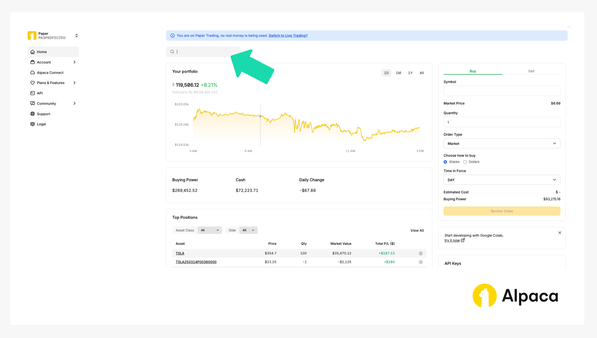
Sign in to your account and navigate to the “Home” page.
Step 2. Find your desired trade
On your dashboard in the top left, we can select between using your paper trading or live accounts. It’s important that we select the appropriate trading account before implementing an options strategy. If we want to practice without the risk of real capital, we can use your paper trading accounts. If we are looking to implement strategies, we can use your live account.
Once you’ve selected the desired account within your dashboard, we can monitor your portfolio, access market data, execute trades, and review your trading history. In order to create your first options trade, use the search bar to find and select the applicable option ticker symbol.
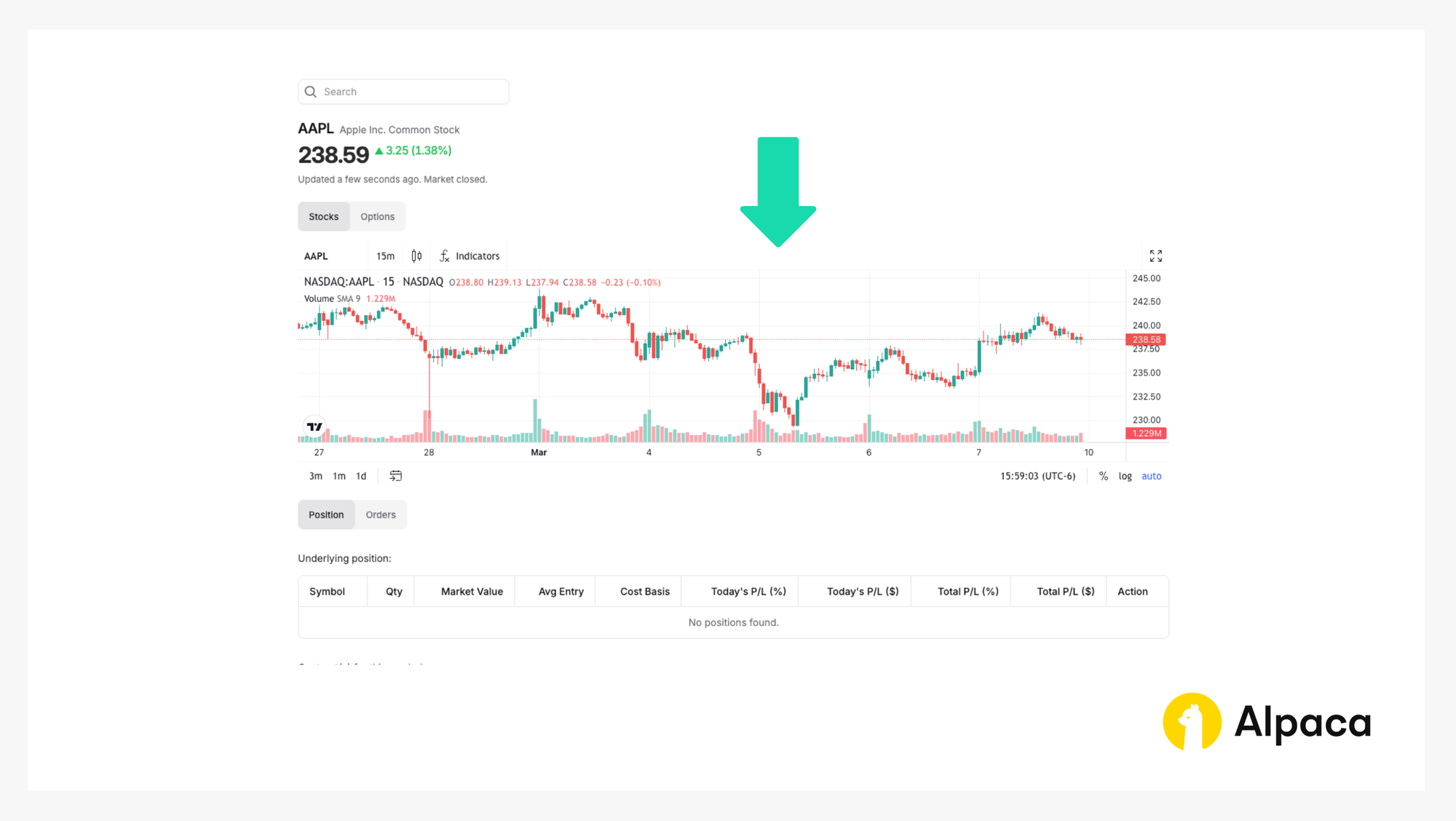
Step 3. Check underlying security’s bar chart
If we search the desired underlying asset, a page shows the asset’s bar chart. We can use this bar chart for a simple analysis.
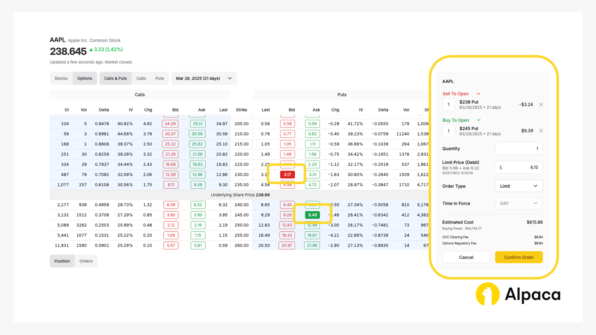
Step 4. Opening an options position
Assume we have already analyzed the market and determined the strike price for the two legs as follows: short put option to be $230.00 and long put to be $245.00 at the expiration date of March 28, 2025. Once determined, select and review your order type (market or limit) and decide on the number of contracts you’d like to trade. We can select up to four legs but in the bear put spread we only need two.
On the asset’s page, toggle from “Stocks” to “Options” and determine your desired contract type between calls and puts. We can also adjust the expiration date from the dropdown, ranging anywhere from 0DTE options to contracts hundreds of days in the future.
A bear put spread, for example, requires longing ITM put options and shorting OTM put options. Therefore, we can establish your position in the dashboard by selecting one short put option with “Sell To Open” and one long put option with "Buy To Open” to purchase the options contracts.
Please note: The order in which we select the options does not matter. Additionally, on Alpaca’s dashboard and Trading API, credits are displayed as negative values, while debits appear as positive values. For example, in the image below, a debit spread (where your initial entry requires payment) is shown with a positive limit price ($6.15 in this case) under 'Limit Price (Debit),' reflecting a total debit of $615.08 (with the additional costs coming from the OCC Clearing Fee and Options Regulatory Fee).
Once selected, review your order type (such as market, limit, stop, stop limit, or trailing stop) and the number of contracts you’d like to trade. Click the “Confirm Order” button on the bottom right.
Your paper trading account will then mimic the execution of the order as though it were a real transaction.
Optional: Cancel your order
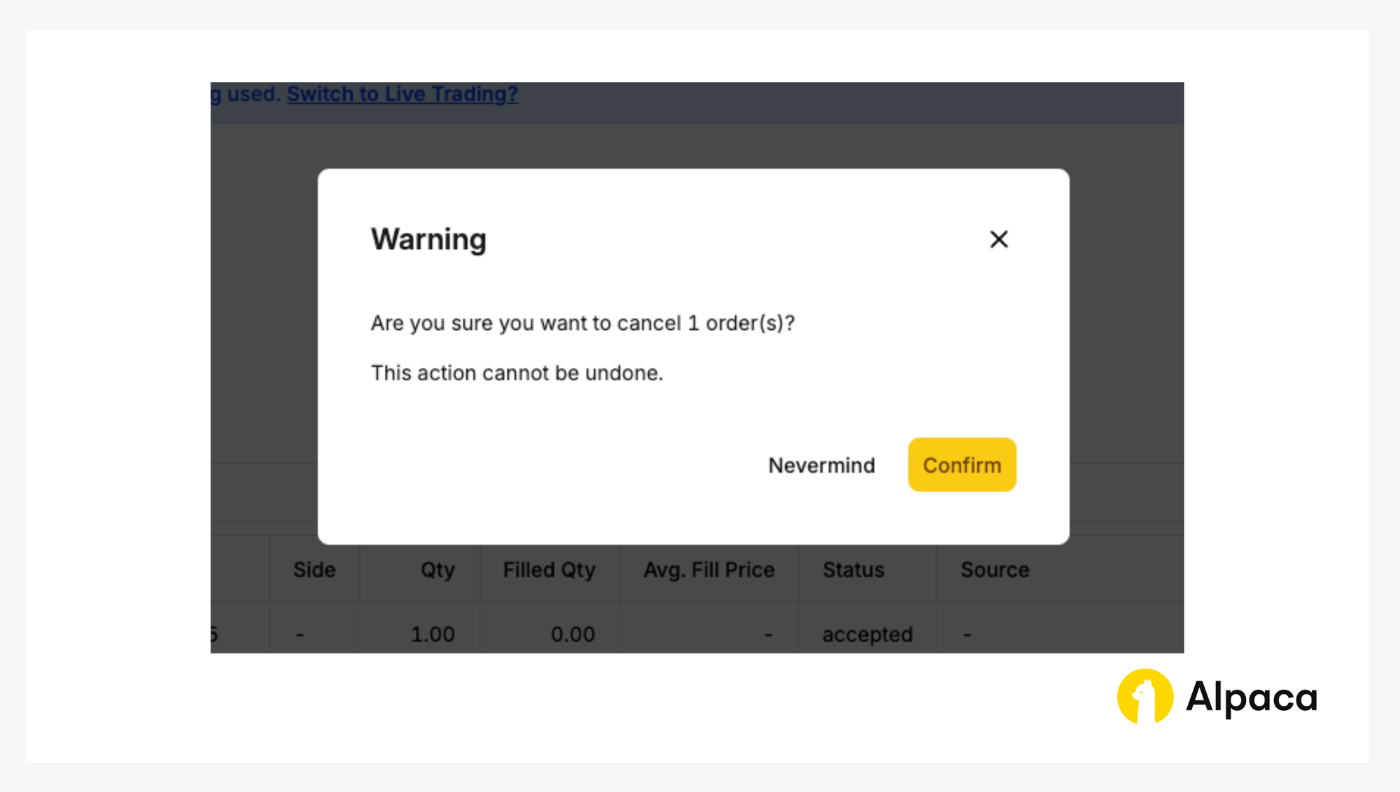
Keep in mind that with a multi-leg options order, we cannot cancel or replace an individual child leg. We can only cancel or replace the entire multi-leg options order. To do this, navigate to the 'Order' section, select the order we want to cancel, and click the 'Cancel 1 selected' button.
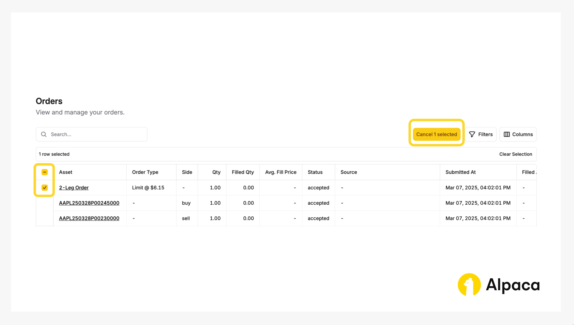
You’ll then be prompted to confirm.
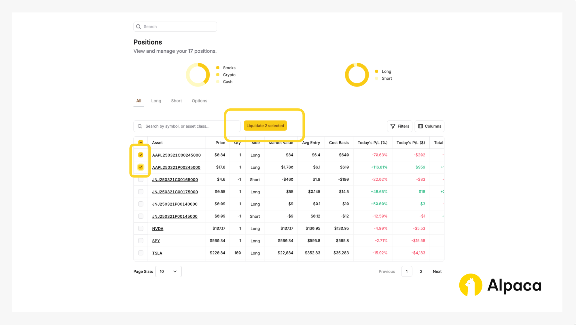
Step 5. Closing your position
Closing an options position involves selling the options contract that we previously bought (in a long position) or buying back the options contract that we previously sold (in a short position). Either action terminates, or “closes”, your associated position.
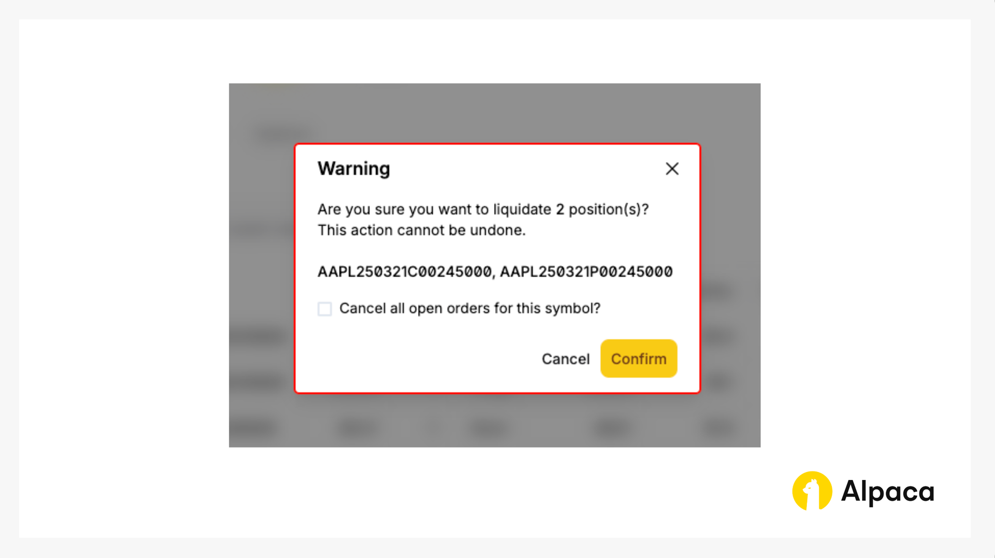
If you’d like to close your position, find the desired options contract on your “Home” page or under “Positions”. Click on the appropriate contract symbol and select “Liquidate 2 selected” to close your bear put spread position.
We will, then, click the “Confirm” button to liquidate the position.
Conclusion
The bear put spread is a structured strategy for traders looking to manage risk while positioning for a moderate decline in an underlying asset’s price. By combining a long put and short put with the same expiration, this spread lowers the upfront cost compared to buying a standalone put while still allowing participation in downward price movements.
As part of a diversified trading approach, the bear put spread can help balance risk and reward, but it requires careful consideration of several factors. Traders should be particularly mindful of implied volatility, the impact of time decay (theta), and how the underlying asset’s price movement aligns with the selected strike prices.
For traders using algorithmic strategies, the bear put spread can be an effective way to express a moderately bearish view while maintaining defined risk parameters. However, as with any options strategy, successful automation requires robust risk management, real-time monitoring, and clear exit criteria. Traders should ensure that their algorithms account for changes in volatility, early assignment risks, and evolving market conditions to enhance long-term performance.
We hope you've found this tutorial on how to trade bear put spreads insightful and useful for getting started on your own strategy. As we put these concepts into practice, feel free to share your feedback and experiences on our forum, Slack community, or subreddit! And don’t forget to check out the rest of our options-related tutorials.
For those looking to integrate options trading with Alpaca’s Trading API, here are some additional resources:
- Sign up for an Alpaca Trading API account
- How to Connect to Alpaca's Trading API
- How to Start Paper Trading with Alpaca's Trading API
- How to Trade Options with Alpaca’s Trading API
- Read more Options Trading Tutorials
- Documentation: Options Trading
Frequently Asked Questions
Is a put spread bullish or bearish?
A bear put spread is a bearish options strategy. It involves purchasing a put option at a higher strike price while simultaneously selling another put option at a lower strike price, both with the same expiration date. This strategy profits when the underlying asset's price declines.
What is the maximum loss on a bear put spread?
The theoretical maximum loss on a bear put spread occurs if the underlying asset's price is at or above the higher strike price at expiration. In this scenario, both put options expire worthless, and the trader incurs a loss equal to the net premium paid to establish the spread. This net premium is the difference between the premium paid for the long put and the premium received for the short put.
What is the risk of bear put spread assignment?
Bear put spreads generally have limited risk of early assignment. This is because the short put option (the one sold) is typically out-of-the-money when the underlying asset's price is above the lower strike price, making early exercise less likely. However, if the underlying asset's price falls below the lower strike price before expiration, the short put could be assigned early, obligating the trader to buy the underlying asset at the short put's strike price. To mitigate this risk, traders should monitor their positions, especially as expiration approaches or if the underlying asset's price moves significantly. In the event of early assignment of the short put, the long put can be exercised to mitigate potential losses, effectively offsetting the cost of assignment.
Options trading is not suitable for all investors due to its inherent high risk, which can potentially result in significant losses. Please read Characteristics and Risks of Standardized Options before investing in options.
Past hypothetical backtest results do not guarantee future returns, and actual results may vary from the analysis.
The Paper Trading API is offered by AlpacaDB, Inc. and does not require real money or permit a user to transact in real securities in the market. Providing use of the Paper Trading API is not an offer or solicitation to buy or sell securities, securities derivative or futures products of any kind, or any type of trading or investment advice, recommendation or strategy, given or in any manner endorsed by AlpacaDB, Inc. or any AlpacaDB, Inc. affiliate and the information made available through the Paper Trading API is not an offer or solicitation of any kind in any jurisdiction where AlpacaDB, Inc. or any AlpacaDB, Inc. affiliate (collectively, “Alpaca”) is not authorized to do business.
Please note that this article is for general informational purposes only and is believed to be accurate as of the posting date but may be subject to change. The examples above are for illustrative purposes only.
All investments involve risk, and the past performance of a security, or financial product does not guarantee future results or returns. There is no guarantee that any investment strategy will achieve its objectives. Please note that diversification does not ensure a profit, or protect against loss. There is always the potential of losing money when you invest in securities, or other financial products. Investors should consider their investment objectives and risks carefully before investing.
Securities brokerage services are provided by Alpaca Securities LLC ("Alpaca Securities"), member FINRA/SIPC, a wholly-owned subsidiary of AlpacaDB, Inc. Technology and services are offered by AlpacaDB, Inc.
This is not an offer, solicitation of an offer, or advice to buy or sell securities or open a brokerage account in any jurisdiction where Alpaca Securities are not registered or licensed, as applicable.