A calendar spread is a strategy where a trader simultaneously sells a short-term option and buys a longer-term option of the same type with the same strike price. The key objective is to benefit from the differential in time decay (theta) and implied volatility between the two legs.

Whether you're looking to understand the theory or looking to implement the strategy with Alpaca either algorithmically or through our dashboard, this tutorial is designed for both audiences. By combining theoretical foundations with actionable strategies for algorithmic integration, you'll gain a comprehensive understanding of calendar spreads and learn how to navigate their complexities for more informed decision-making in the options market.

This introduction will explore the mechanics of calendar spreads, offering a clear breakdown of how these strategies operate and the risk-reward trade-offs they entail. Transparency is key when evaluating derivatives strategies—so this guide highlights both opportunities and risks to help traders make informed decisions.

What is a Calendar Spread?

A calendar spread is an options strategy that involves selling a short-term option while simultaneously purchasing a longer-term option of the same type (call or put) and at the same strike price. Both options are also based on the same underlying stock or ETF. This strategy is also known as a time spread or horizontal spread.

The term calendar spread refers to the position's value being influenced by the difference in option Greeks like time decay (theta) and implied volatility (vega) between the two options over the time period. The short-term option, often called the front-month or near-term option, has an earlier expiration, while the longer-term option is known as the back-month option.

When to Use a Calendar Spread?

Calendar spreads are often used to seek potential income. Traders use calendar spreads to capitalize on differences in the time decay of options or passage of time rather than directional price movement alone, like a delta neutral strategy, while offering a defined risk profile.

Specifically, the goal of calendar spreads would be slightly differ depending on the types of structures.

• Long Calendar Spreads: Profit from time decay and potential increases in implied volatility. Traders may expect the underlying asset to remain near the strike price until the near-term option expires. If the value of the combined spread increases, you may attempt to sell it for a profit before the short call or put expires.
• Short Calendar Spreads: Profit from rapid time decay and decreasing implied volatility. The trader may also possibly benefit if the underlying asset moves significantly away from the strike price. If the value of the combined spread decreases, you may attempt to buy to close it for a profit before the long call or put expires.

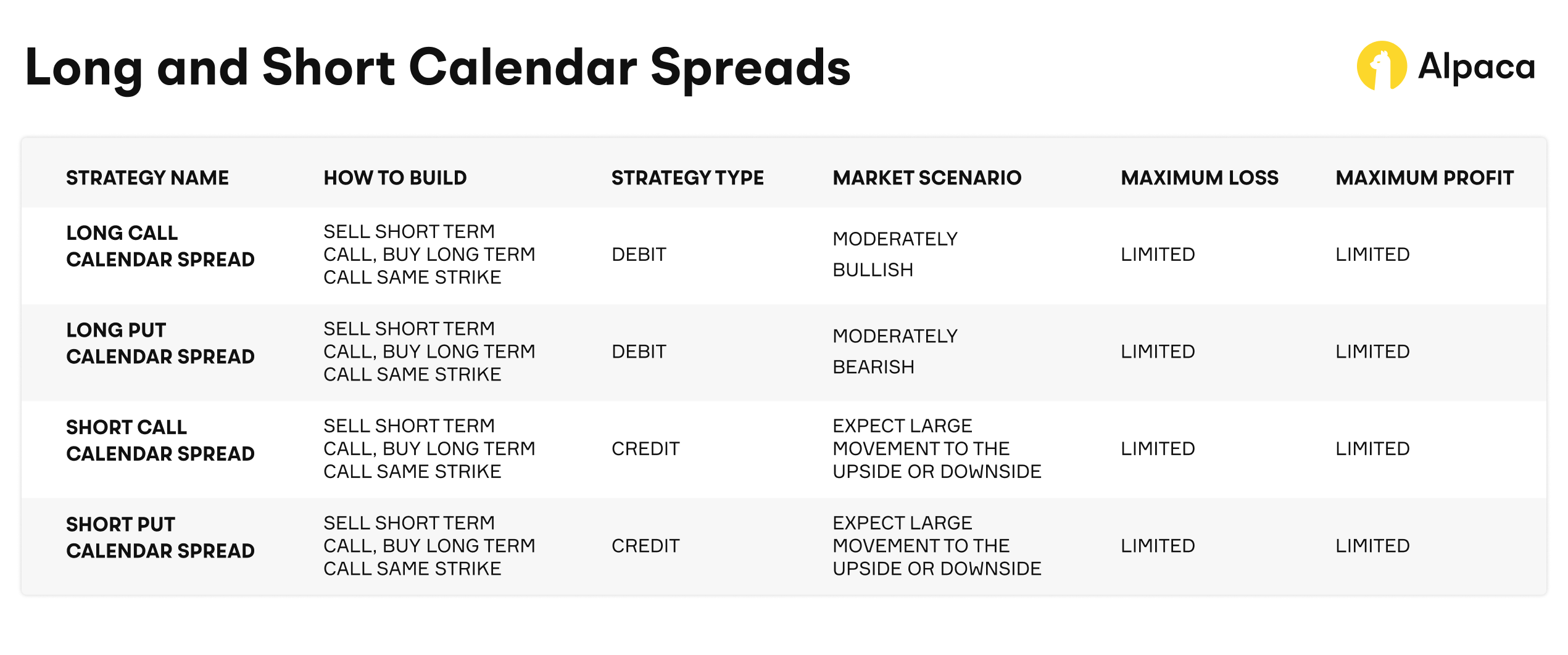
The Different Types of Calendar Spreads

As shown above, there are two categories of calendar spreads: long calendar spreads and short calendar spreads. Between those categories, there are four overall types: long call calendar spreads, long put calendar spreads, short call calendar spreads, and short put calendar spreads. We will break down each type below.

Long Call Calendar Spread

The long call calendar spread is a neutral to mildly bullish strategy involving the purchase of a longer-term call and the sale of a shorter-term call at the same strike. The goal of this type of calendar spread is to capitalize on the faster time decay of the shorter-term call while retaining bullish exposure via the longer-term call.

When to Use It

• Price Expectation: You anticipate the underlying will remain near or slightly above the strike price.
• Volatility Expectation: Slight increase or stable implied volatility over time.
• Time Horizon: The near-term call expiration in a few weeks; the long-term call might expire in a few months.

Building the Strategy

Here is the basic structure to build the long call calendar spread.

• Buy (long) a longer-term call option.
• Sell (short) a shorter-term call option (at the same strike price).
• Profitability: Typically optimized when the underlying price remains stable and volatility increases.

Long Put Calendar Spread

A long put calendar spread is a neutral to mildly bearish strategy that involves purchasing a longer-term put option and selling a shorter-term put option at the same strike price. This strategy aims to take advantage of the faster time decay of the short-term put while maintaining downside exposure through the longer-term put.

When to Use It

• Price Expectation: You anticipate the underlying price will remain near or slightly below the strike price.
• Volatility Expectation: You expect implied volatility to increase or remain stable.
• Time Horizon: The near-term put expires in a few weeks, while the longer-term put expires in a few months.

Building the Strategy

Here is the basic structure to build the long put calendar spread:

• Buy a longer-term put option.
• Sell a shorter-term put option (at the same strike price).
• Profitability: There is profit potential if the underlying price remains stable or declines while volatility increases.

Short Call Calendar Spread

A short call calendar spread is a neutral to slightly bearish strategy that involves selling a longer-term call option while buying a shorter-term call option at the same strike price. The goal is to potentially benefit from the faster decay of the short-term call while managing risk through the longer-term call.

When to Use It

• Price Expectation: You anticipate the underlying will stay near or below the strike price.
• Volatility Expectation: You expect implied volatility to decrease.
• Time Horizon: The near-term call expires within a few weeks, while the longer-term call expires in a few months.

Building the Strategy

Here is the basic structure to build the short call calendar spread:

• Sell a longer-term call option.
• Buy a shorter-term call option (at the same strike price).
• Profitability: Beneficial if volatility remains low and the underlying price is range-bound or declines.

Short Put Calendar Spread

A short put calendar spread is a neutral to slightly bullish strategy that involves selling a longer-term put option while buying a shorter-term put option at the same strike price. This setup profits if the underlying price remains stable or rises, and if implied volatility decreases.

When to Use It

• Price Expectation: You anticipate the underlying will stay near or above the strike price.
• Volatility Expectation: You expect implied volatility to decrease.
• Time Horizon: The near-term put expires in a few weeks, while the longer-term put expires in a few months.

Building the Strategy

Here is the basic structure to build the short put calendar spread:

• Sell a longer-term put option.
• Buy a shorter-term put option (same strike price).
• Profitability: Effective if the underlying asset remains stable or rises in value, and if volatility drops.

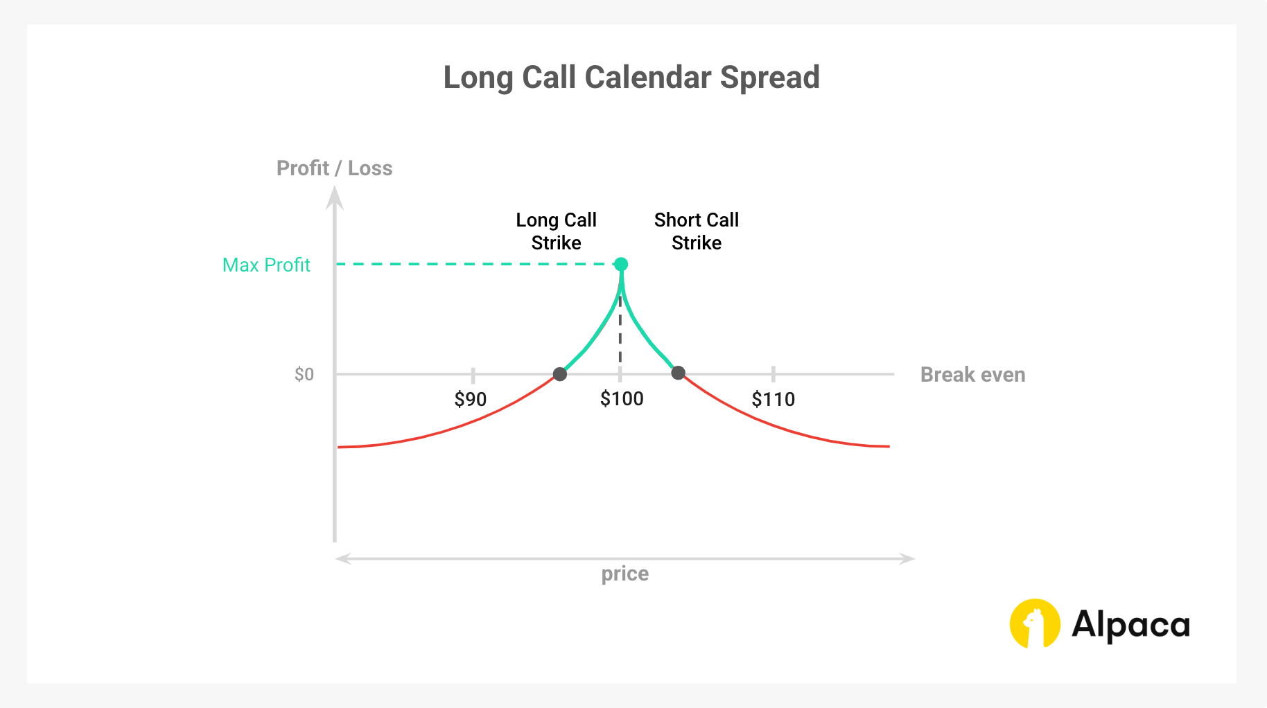
Example: Long Call Calendar Spread (with Payoff Diagram)

To illustrate how a calendar spread performs under different market conditions, let's analyze a long call calendar spread using XYZ stock as the underlying asset. Please note that breakeven points for a long call calendar spread depend on expiration dates and implied volatility, making them harder to calculate than single-option strategies. In our comprehensive article on Level 3 options trading strategies, we have covered both long and short call calendar spreads.

Example Setup:

• Underlying Price: XYZ is trading at $100.
• Sell: 1 XYZ call, strike $100, expiring in 1 month (short-term), premium = $2.50 ($250 total).
• Buy: 1 XYZ call, strike $100, expiring in 3 months (long-term), premium = $5.00 ($500 total).
• Net Debit: -$500 (long call) + $250 (short call) = -$250 (theoretical maximum possible loss).

Scenario 1: XYZ is at $100 at the time of the short call’s expiration.

• The short call expires worthless and you keep the $250 premium.
• The long call still has a time value. Potential profit depends on how the long call is priced at that point.

Scenario 2: XYZ is at $110 at the time of the short call’s expiration.

• Short call is in-the-money (ITM) and has the risk of early assignment.
• You could exercise or sell the long call to manage the assignment.
• It would be safe to compare the market price of the long call (intrinsic + time value) to its intrinsic value alone.
  • If the long call has little or no remaining time value (extrinsic value), exercise it to acquire the shares at $100 and reduce your total loss.
  • If the long call retains significant time value, sell it in the market to capture its full premium. Then, use the proceeds to manage the assignment
• Theoretical profit or loss:  If you exercise the long call, the loss from buying and selling the XYZ shares becomes $0, but the initial loss of $250 may remain as your total loss.

Scenario 3: XYZ is at $90 at the time of the short call’s expiration.

• Both calls are out-of-the-money (OTM).
• Short call expires worthless while your long call has decreased in value.
• Final loss depends on the residual value of the long call.

Factors That Affect Calendar Spreads

Many of the factors that affect calendar spreads can be explained by option Greeks. Each impacts the calendar spread slightly differently, depending on whether it is a short or long calendar spread.

Time Decay (Theta Decay – How Time Erodes Value)

• Long Calendar Spreads:
  • Typically benefit from time decay because the short-term option often loses value faster than the long-term option.
  • If the underlying price stays near the strike, the short option expires worthless.
  • After the short option expires, the remaining long option starts losing value faster, requiring active management.
• Short Calendar Spreads:
  • Affected by time decay, the short-term option (which the trader owns) loses value quickly. This may reduce net profit because, by the time traders want to sell the short-term option, its value has diminished.
  • The longer-term option (which the trader sold) holds its value, potentially making the position less profitable.

Implied Volatility (Vega – How Volatility Affects the Spread)

• Long Calendar Spreads:
  • Gain potential profit when volatility increases because the long-term option becomes more valuable.
  • Work well when volatility is low at entry and expected to rise, as this increases the premium of the long-term option, leading to a higher net potential profit.
  • Risky if volatility drops after entry, as the spread will shrink in value.
• Short Calendar Spreads:
  • May experience a reduction in potential profit when volatility increases because the short-term option can gain value quickly.
  • Work well when volatility is high at entry and expected to fall, as this diminishes the cost to buy back the long-term option, leading to a higher net potential profit.
  • Risky if volatility rises unexpectedly, making the short-term option expensive.

Price Movement Risk (Gamma – How Stock Price Changes Impact the Spread)

• Long Calendar Spreads:
  • Best when the stock stays near the strike price of the short-term option.
  • If the stock moves too much, the strategy loses effectiveness, and adjustments may be needed.
• Short Calendar Spreads:
  • Best when the stock moves significantly in either direction.
  • If the stock stays still, the trade possibly loses value as time decay hurts the short-term option more than expected.

The Advantages and Disadvantages of Calendar Spreads

Just as any other option strategies, calendar spreads have advantages and disadvantages. Here are the main pros and cons of the strategy.

Advantages of Calendar Spreads

While each type of calendar spreads has slight nuances, they generally share similar advantages.

• Defined Risk Exposure: Losses are generally limited to the initial cost of the trade, which provides a structured-risk approach.
• Theta Arbitrage: Traders may benefit from the short-term option potentially decaying faster than the long-term option.
• Volatility Flexibility: Calendar spreads potentially do well in conditions of changing implied volatility over the time period, making them useful in uncertain markets.
• Low Capital Requirement: In many cases, the cost of calendar spreads, even debit spreads, can be lower than outright long options strategies.
• Algorithmic Optimization: The spread’s behavior under various volatility and decay conditions makes it suitable for systematic strategies.

Disadvantages of Calendar Spreads

Just as calendar spreads share common advantages, they also expose traders to similar risks.

• Limited Profit Potential: Unlike directional strategies, profit is capped at the difference between the two legs.
• Liquidity Risks: Longer-term options often have wider bid-ask spreads, affecting execution quality. Additionally, calendar spreads possibly become challenging in low-liquidity options markets, making it harder to exit at favorable prices.
• Risk of Early Exercise (for American-Style Options): If the short option is exercised early, the spread structure collapses, requiring immediate position management.
• Dividend Assignment Risk: Early assignment risk increases on a stock’s ex-dividend date, especially for short call options, as holders may exercise to profit from the dividend-premium difference
• Sensitivity to Implied Volatility Changes: A drop in implied volatility would lead to a potential loss sometimes, particularly if executed near an earnings event or major economic release. Though unlikely, if volatility does not behave as expected, the long leg may lose value faster than anticipated, increasing risk due to decay mismatch.
• Complex Position Management: Adjustments may be required if the underlying asset moves too far from the strike price.
• Vulnerability to Large Price Moves: In a long calendar spread, a significant move in the underlying asset in either direction may cause the spread to lose value.

Executing a Calendar Spread Using Alpaca’s Trading API

This section provides a step-by-step guide to implementing a long call calendar spread using Python and Alpaca’s Trading API in the Paper Trading environment. The strategy involves selling a near-term at-the-money (ATM) call option while simultaneously buying a longer-term call option at the same strike price. This approach helps manage risk and optimize decision-making by leveraging key metrics and filters. If you’re not connected to Alpaca’s API, sign up and learn how to start paper trading with Alpaca.

Important Notes:

• The code assumes a flat interest rate, excludes dividends, and is not optimized for 0DTE options. It does not consider market hours and serves as a starting point rather than a complete strategy.
• Expiration Day Order Rules:
  • Orders must be submitted before 3:15 p.m. ET for stocks/options and 3:30 p.m. ET for broad-based ETFs (e.g., SPY, QQQ).
  • Orders placed after these times will be rejected.
  • Expiring positions are auto-liquidated at 3:30 p.m. ET (stocks/options) and 3:45 p.m. ET (broad-based ETFs) for risk management.
• Multi-Leg (MLeg) Orders:
  • All legs of a strategy must be included in the same order for acceptance.
  • This is crucial for strategies with uncovered short options (e.g., short put calendar spreads, short call calendar spreads), which require Level 4 approval. See Alpaca's multi-leg order restrictions for details.
• American-Style Options Considerations:
  • American-style options may be assigned early, affecting trade outcomes. Profit/loss scenarios assume expiration without early exercise and do not factor in transaction fees (e.g., brokerage fees, commissions). Traders should also monitor ex-dividend dates for short calls to manage assignment risk.
• Example equity:
  • "AA" is used for demonstration purposes and should not be considered investment advice.

Setting Up the Environment and Trade Parameters

The first step involves configuring the environment for trading a calendar spread option and specifying your Alpaca Paper Trading API keys. This ensures your API connections and variable setup are secure and streamlined for data retrieval and trading operations. 

Note: While we are using Jupyter Notebook for this tutorial, you can use Google Collab or any other IDE as your code environment. You can also find all of the below code on Alpaca’s Github page.

!python3 -m pip install --upgrade alpaca-py
import pandas as pd
import numpy as np
from scipy.stats import norm
import alpaca
import time
from scipy.optimize import brentq
from datetime import datetime, timedelta
from zoneinfo import ZoneInfo
from alpaca.data.timeframe import TimeFrame, TimeFrameUnit
from dotenv import load_dotenv
import os

from alpaca.data.historical.option import OptionHistoricalDataClient
from alpaca.data.historical.stock import StockHistoricalDataClient, StockLatestTradeRequest
from alpaca.data.requests import StockBarsRequest, OptionLatestQuoteRequest, OptionChainRequest, OptionBarsRequest
from alpaca.trading.client import TradingClient
from alpaca.trading.requests import (
    MarketOrderRequest,
    GetOptionContractsRequest,
    MarketOrderRequest,
    OptionLegRequest,
    ClosePositionRequest,
)
from alpaca.trading.enums import (
    AssetStatus,
    ExerciseStyle,
    OrderSide,
    OrderClass,
    OrderStatus,
    OrderType,
    TimeInForce,
    QueryOrderStatus,
    ContractType,
)

The script initializes Alpaca clients for trading stocks and options, as well as for handling data requests.

# API credentials for Alpaca API
API_KEY = "YOUR_ALPACA_API_KEY_FOR_PAPER_TRADING"
API_SECRET = 'YOUR_ALPACA_API_SECRET_KEY_FOR_PAPER_TRADING'
BASE_URL = None
## We use a paper environment for this example (Please do not modify this. This example is for paper trading only)
PAPER = True

# Initialize Alpaca clients
trade_client = TradingClient(api_key=API_KEY, secret_key=API_SECRET, paper=PAPER, url_override=BASE_URL)
option_historical_data_client = OptionHistoricalDataClient(api_key=API_KEY, secret_key=API_SECRET, url_override=BASE_URL)
stock_data_client = StockHistoricalDataClient(api_key=API_KEY, secret_key=API_SECRET)

# Below are the variables for development this documents
# Please do not change these variables
trade_api_url = None
trade_api_wss = None
data_api_url = None
option_stream_data_wss = None

Choosing the Right Strike Price and Expiration

Selecting an appropriate strike price and expiration is crucial for optimizing a long calendar spread. Each choice influences risk, profitability, and trade efficiency.

• Strike Price Selection Using Option Moneyness:
  • ATM options are typically preferred since they balance premium collection with manageable risk.
  • OTM options may offer lower costs but require a significant price move to be profitable.
  • ITM options have higher premiums and intrinsic value but reduce the benefit of time decay.
• Expiration Timing:
  • The short leg is set to expire sooner (27-40 days) to capture rapid theta decay and premium collection.
  • The long leg is chosen with a longer expiration (55-65 days) to provide flexibility for adjustments and potentially benefit from potential volatility shifts.
  • This expiration structure ensures that the strategy effectively captures time decay on the short leg while maintaining exposure to price movements.

Factor in Risk Management and Position Sizing

Proper risk management and position sizing may help optimize returns while limiting downside risk. With this approach, the algorithm dynamically adjusts trade size based on market conditions, volatility, and liquidity constraints. Below are some of the factors we considered when writing the strategy:

Adaptive Position Sizing

The trade size is adjusted based on market conditions, ensuring that capital allocation remains optimal relative to volatility and risk exposure. Key factors influencing position sizing include:

• Buying Power Allocation: The strategy limits allocation to 5% of available buying power, attempting to prevent over-leverage.
• Strike Price Range: To ensure liquidity and trade viability, the system filters strikes within a 3% range above and below the underlying price.
• Expiration Selection: The short-leg option is chosen with an expiration of 27-40 days, while the long-leg option is selected between 55-65 days, potentially allowing for an optimal balance between premium collection and theta decay.
• Liquidity Check: The algorithm only selects options with at least 200 open interest, ensuring sufficient market depth to enter and exit positions efficiently.

Stop-Loss Mechanisms

To minimize drawdowns, the algorithm integrates automated stop-loss features:

• Volatility-Based Exit: If implied volatility (IV) shifts significantly beyond expected levels (short-leg IV: 40-70%, long-leg IV: 30-60%), the system can trigger an exit to avoid excessive risk exposure.
• Greek-Based Thresholds: The strategy monitors delta (short-leg: 0.45-0.80, long-leg: 0.40-0.70) and theta (short-leg: -0.2 to -0.01, long-leg: -0.1 to -0.01) to manage risk from rapid time decay and directional movement.
• Profit Target Exit: Positions are exited if the trade achieves 40% of the target profit, ensuring gains are locked in before market conditions shift.
• Hard Cutoff Risk Management: Since Alpaca enforces an early order submission cutoff (3:15 p.m. ET for stocks/options, 3:30 p.m. ET for ETFs), trades are monitored for auto-liquidation risk, ensuring no unwanted expirations.

By incorporating these adaptive risk management techniques, the strategy effectively balances risk and reward while maintaining liquidity and market adaptability.

# Select the underlying stock (Alcoa Corporation)
underlying_symbol = 'AA'

# Set the timezone
timezone = ZoneInfo("America/New_York")

# Get current date in US/Eastern timezone
today = datetime.now(timezone).date()

# Define a 5% range around the underlying price 
STRIKE_RANGE = 0.05

# Buying power percentage to use for the trade
BUY_POWER_LIMIT = 0.05

# Risk free rate for the options greeks and IV calculations
risk_free_rate = 0.01

# Check account buying power
buying_power = float(trade_client.get_account().buying_power)

# Set the open interest volume threshold
OI_THRESHOLD = 100

# Calculate the limit amount of buying power to use for the trade
buying_power_limit = buying_power * BUY_POWER_LIMIT

# Set the expiration date range for the options
min_expiration = today + timedelta(days=21)
max_expiration = today + timedelta(days=80)

# Get the latest price of the underlying stock
def get_underlying_price(symbol):
    # Get the latest trade for the underlying stock
    underlying_trade_request = StockLatestTradeRequest(symbol_or_symbols=symbol)
    underlying_trade_response = stock_data_client.get_stock_latest_trade(underlying_trade_request)
    return underlying_trade_response[symbol].price

# Get the latest price of the underlying stock
underlying_price = get_underlying_price(underlying_symbol)

# Set the minimum and maximum strike prices based on the underlying price
min_strike = str(underlying_price * (1 - STRIKE_RANGE))
max_strike = str(underlying_price * (1 + STRIKE_RANGE))

# Define expiry thresholds. For a shorter-term call, between 27 days and 40 days, which is buffer for 30 days; for a longer-term, between 55 days and 65 days, which is buffer for 60 days
EXPIRY_RANGE = (27, 40, 55, 65)

# Define Implied Volatility thresholds. For a shorter-term call, between 0.40 and 0.70; for a longer-term, between 0.30 and 0.60
IV_RANGE = (0.40, 0.70, 0.30, 0.60)

# Define delta thresholds. For a shorter-term call, between 0.45 and 0.80; for a longer-term, between 0.40 and 0.70
DELTA_RANGE = (0.45, 0.80, 0.40, 0.70)

# Define theta thresholds. For a shorter-term call, between -0.2 and -0.01; for a longer-term, between -0.1 and -0.01
THETA_RANGE = (-0.2, -0.01, -0.1, -0.01)

# Set target profit levels
TARGET_PROFIT_PERCENTAGE = 0.6

# Display the values
print(f"Underlying Symbol: {underlying_symbol}")
print(f"{underlying_symbol} price: {underlying_price}")
print(f"Strike Range: {STRIKE_RANGE}")
print(f"Buying Power Limit Percentage: {BUY_POWER_LIMIT}")
print(f"Risk Free Rate: {risk_free_rate}")
print(f"Account Buying Power: {buying_power}")
print(f"Buying Power Limit: {buying_power_limit}")
print(f"Open Interest Threshold: {OI_THRESHOLD}")
print(f"Minimum Expiration Date: {min_expiration}")
print(f"Maximum Expiration Date: {max_expiration}")
print(f"Minimum Strike Price: {min_strike}")
print(f"Maximum Strike Price: {max_strike}")
print(f"Expiry date range for options: {EXPIRY_RANGE}")
print(f"Implied Volatility range for options: {IV_RANGE}")
print(f"Delta range for options: {DELTA_RANGE}")
print(f"Theta range for options: {THETA_RANGE}")

Calculations for Implied Volatility and Option Greeks with Black-Scholes model

The calculate_implied_volatility function estimates implied volatility (IV) using the Black-Scholes model. The function defines a reasonable range for sigma (1e-6 to 5.0) to avoid extreme values. For deep OTM options where the price is close to intrinsic value, the function directly sets IV to 0.0 to prevent calculation errors. A numerical root-finding method is used to solve for IV, ensuring accuracy even in edge cases.

# Calculate implied volatility
def calculate_implied_volatility(option_price, S, K, T, r, option_type):
    
    # Define a reasonable range for sigma
    sigma_lower = 1e-6
    sigma_upper = 5.0  # Adjust upper limit if necessary

    # Check if the option is out-of-the-money and price is close to zero
    intrinsic_value = max(0, (S - K) if option_type == 'call' else (K - S))
    if option_price <= intrinsic_value + 1e-6:
        
        # print("Option price is close to intrinsic value; implied volatility is near zero.") # Uncomment for checking the status
        return 0.0
    
    # Define the function to find the root
    def option_price_diff(sigma):
        d1 = (np.log(S / K) + (r + 0.5 * sigma ** 2) * T) / (sigma * np.sqrt(T))
        d2 = d1 - sigma * np.sqrt(T)
        if option_type == 'call':
            price = S * norm.cdf(d1) - K * np.exp(-r * T) * norm.cdf(d2)
        elif option_type == 'put':
            price = K * np.exp(-r * T) * norm.cdf(-d2) - S * norm.cdf(-d1)
        return price - option_price

    try:
        return brentq(option_price_diff, sigma_lower, sigma_upper)
    except ValueError as e:
        print(f"Failed to find implied volatility: {e}")
        return None

The calculate_greeks function estimates all option Greeks: delta, gamma, theta, and vega based on the implied volatility calculated through calculate_implied_volatility. In this demonstration, we mainly use delta and theta as well as implied volatility.

def calculate_greeks(option_price, strike_price, expiry, underlying_price, risk_free_rate, option_type):
    T = (expiry - pd.Timestamp.now()).days / 365 # It is unconventional, but some use 225 days (# of annual trading days) in replace of 365 days
    T = max(T, 1e-6)  # Set minimum T to avoid zero
    
    if T == 1e-6:
        print("Option has expired or is expiring now; setting Greeks based on intrinsic value.")
        if option_type == 'put':
            delta = -1.0 if underlying_price < strike_price else 0.0
        else:
            delta = 1.0 if underlying_price > strike_price else 0.0
        gamma = 0.0
        theta = 0.0
        vega = 0.0
        return delta, gamma, theta, vega
    
    # Calculate IV
    IV = calculate_implied_volatility(option_price, underlying_price, strike_price, T, risk_free_rate, option_type)
    print(f"implied volatility is {IV}")
    if IV is None or IV == 0.0:
        print("Implied volatility could not be determined, skipping Greek calculations.")
        return None
    
    d1 = (np.log(underlying_price / strike_price) + (risk_free_rate + 0.5 * IV ** 2) * T) / (IV * np.sqrt(T))
    d2 = d1 - IV * np.sqrt(T) # d2 for Theta calculation
    # Calculate Delta
    delta = norm.cdf(d1) if option_type == 'call' else -norm.cdf(-d1)
    # Calculate Gamma
    gamma = norm.pdf(d1) / (underlying_price * IV * np.sqrt(T))
    # Calculate Vega
    vega = underlying_price * np.sqrt(T) * norm.pdf(d1) / 100
    # Calculate Theta
    if option_type == 'call':
        theta = (
            - (underlying_price * norm.pdf(d1) * IV) / (2 * np.sqrt(T))
            - (risk_free_rate * strike_price * np.exp(-risk_free_rate * T) * norm.cdf(d2))
        )
    else:
        theta = (
            - (underlying_price * norm.pdf(d1) * IV) / (2 * np.sqrt(T))
            + (risk_free_rate * strike_price * np.exp(-risk_free_rate * T) * norm.cdf(-d2))
        )
    # Convert annualized theta to daily theta
    theta /= 365
    
    return delta, gamma, theta, vega

Factors To Include In Your Strategy

When implementing a long calendar spread, it's essential to identify market conditions that support this strategy. Using a combination of price trends, volatility measures, and technical indicators, traders would be able to optimize entry points and improve trade efficiency. The following factors may help trigger calendar spread setups based on underlying asset price movement and volatility events.

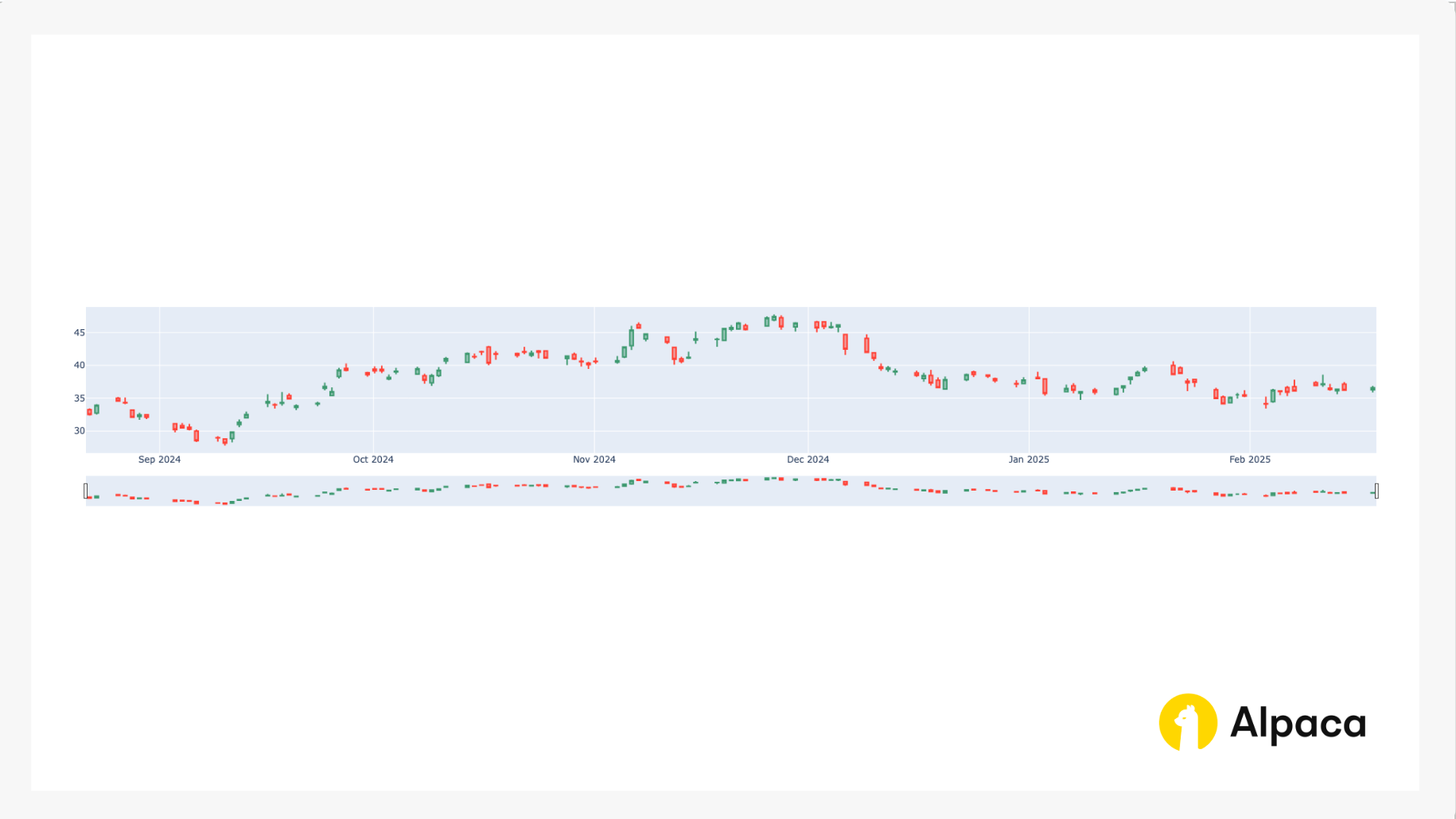
Stock Price Trends (Bar Chart Analysis)

Monitoring historical price movements helps traders assess the broader trend of the underlying asset. A candlestick chart provides insight into recent price action, support, and resistance levels, which may help determine whether the market is range-bound or trending. Calendar spreads work best in low-volatility environments where the underlying asset remains stable within a defined range.

# Get the historical data for the underlying stock by symbol and timeframe
# ref. https://alpaca.markets/sdks/python/api_reference/data/option/historical.html
def get_stock_data(underlying_symbol, days=90):
    today = datetime.now(timezone).date()
    req = StockBarsRequest(
        symbol_or_symbols=[underlying_symbol],
        timeframe=TimeFrame(amount=1, unit=TimeFrameUnit.Day),     # specify timeframe
        start=today - timedelta(days=days),                          # specify start datetime, default=the beginning of the current day.
    )
    return stock_data_client.get_stock_bars(req).df

priceData = get_stock_data(underlying_symbol, days=180)

# List of stock agg objects while dropping the symbol column
priceData = priceData.reset_index(level='symbol', drop=True)

import plotly.graph_objects as go

fig = go.Figure(data=[go.Candlestick(x=priceData.index,
                open=priceData['open'],
                high=priceData['high'],
                low=priceData['low'],
                close=priceData['close'])])

fig.show()

This script returns the bar chart like in the image below.

Relative Volatility Index (RVI)

The RVI indicator measures the strength of price momentum relative to volatility. It helps confirm whether the market is experiencing a period of increased price fluctuations or stabilizing. If the RVI is high, it suggests strong directional movement, which may not be ideal for a neutral calendar spread strategy. Conversely, a low or declining RVI may signal a stable market environment, making it a more favorable setup.

def calculate_rvi(df, period=14):
    # Calculate daily price changes 
    df["price_change"] = df["close"].diff()

    # Separate up and down price changes
    df['up_change'] = df['price_change'].where(df['price_change'] > 0, 0)
    df['down_change'] = -df['price_change'].where(df['price_change'] < 0, 0)

    # Calculate std of up and down changes over the rolling period
    df['avg_up_std'] = df['up_change'].rolling(window=period).std()
    df['avg_down_std'] = df['down_change'].rolling(window=period).std()

    # Calculate RVI
    df['rvi'] = 100 - (100 / (1 + (df['avg_up_std'] / df['avg_down_std'])))

    # Smooth the RVI with a 4 periods moving average
    df['rvi_smoothed'] = df['rvi'].rolling(window=4).mean()

    return df['rvi_smoothed']

# smoothed RVI
calculate_rvi(priceData, period=21).iloc[30:]

Bollinger Bands for Volatility Assessment

Bollinger Bands provide a dynamic range around the asset's price, helping to gauge market volatility. When the underlying stock price is near the upper Bollinger Band, it may indicate overbought conditions, while a price near the lower band suggests oversold levels. 

Calendar spreads potentially benefit from moderate volatility, where prices stay near the middle of the band rather than trending towards extreme levels. If the asset is trading closer to the upper or lower Bollinger Band, adjustments may be needed to avoid an early breakout risk.

# setup bollinger band calculations
def check_bb(df, period=14, multiplier=2):
    bollinger_bands = []
    # Calculate the Simple Moving Average (SMA)
    df['SMA'] = df['close'].rolling(window=period).mean()
    # Calculate the rolling standard deviation
    df['StdDev'] = df['close'].rolling(window=period).std()
    # Calculate the Upper Bollinger Band (two standard deviation)
    df['Upper Band'] = df['SMA'] + (multiplier * df['StdDev'])
    # Calculate the Lower Bollinger Band (two standard deviation)
    df['Lower Band'] = df['SMA'] - (multiplier * df['StdDev'])
    # Get the most recent Upper Band value
    upper_bollinger_band = df['Upper Band'].iloc[-1]
    lower_bollinger_band = df['Lower Band'].iloc[-1]
    
    bollinger_bands = [upper_bollinger_band, lower_bollinger_band]
    return bollinger_bands

bollinger_bands = check_bb(priceData, 14, 2)

print(f"Latest Upper Bollinger Band is: {bollinger_bands[0]}. Latest Lower Bollinger Band is {bollinger_bands[1]}; while underlying stock '{underlying_symbol}' price is {underlying_price}.")

Constructing a Calendar Spread

First, we build the get_call_options function to be able to fetch active call options for a given underlying symbol within the specified strike price and expiration range.

# Check for call options
def get_call_options(underlying_symbol, min_strike, max_strike, min_expiration, max_expiration):
    
    # Fetch the options data to add to the portfolio
    req = GetOptionContractsRequest(
        underlying_symbols=[underlying_symbol],
        status=AssetStatus.ACTIVE,
        type=ContractType.CALL,
        strike_price_gte=min_strike,
        strike_price_lte=max_strike,
        expiration_date_gte=min_expiration,
        expiration_date_lte=max_expiration,
    )
    
    # Get call option chain of the underlying symbol
    call_options = trade_client.get_option_contracts(req).option_contracts
    return call_options

A helper function build_option_dict constructs an option dictionary from option data and its calculated metrics. This is used within thefind_call_options_for_calendar_spread fucntion to store details for both short and long call options.

def build_option_dict(option_data, iv, delta, theta, option_price):
    """
    Helper to build an option dictionary from option_data and calculated metrics.
    """
    return {
        'id': option_data.id,
        'name': option_data.name,
        'symbol': option_data.symbol,
        'strike_price': option_data.strike_price,
        'root_symbol': option_data.root_symbol,
        'underlying_symbol': option_data.underlying_symbol,
        'underlying_asset_id': option_data.underlying_asset_id,
        'close_price': option_data.close_price,
        'close_price_date': option_data.close_price_date,
        'expiration_date': option_data.expiration_date,
        'open_interest': option_data.open_interest,
        'open_interest_date': option_data.open_interest_date,
        'size': option_data.size,
        'status': option_data.status,
        'style': option_data.style,
        'tradable': option_data.tradable,
        'type': option_data.type,
        'initial_IV': iv,
        'initial_delta': delta,
        'initial_theta': theta,
        'initial_option_price': option_price,
    }

The below filters and selects short and long call options for a calendar spread based on criteria like expiration, implied volatility, delta, theta, and open interest.

def find_call_options_for_calendar_spread(call_options, underlying_price, risk_free_rate, buying_power_limit, expiry_range, iv_range, delta_range, theta_range):
    
    short_call = None
    long_call = None

    for option_data in call_options:
        option_symbol = option_data.symbol
        print(f"\nChecking option {option_symbol}...")

        try:
            # Check required fields and open interest
            if option_data.open_interest is None or option_data.open_interest_date is None:
                print(f"Skipping {option_symbol}: missing open_interest or open_interest_date.")
                continue
            if float(option_data.open_interest) <= OI_THRESHOLD:
                print(f"Skipping {option_symbol}: open_interest {option_data.open_interest} is below threshold {OI_THRESHOLD}.")
                continue

            # Get option quote and calculate basic metrics
            option_quote_request = OptionLatestQuoteRequest(symbol_or_symbols=option_symbol)
            option_quote = option_historical_data_client.get_option_latest_quote(option_quote_request)[option_symbol]

            option_price = (option_quote.bid_price + option_quote.ask_price) / 2
            strike_price = float(option_data.strike_price)
            expiry = pd.Timestamp(option_data.expiration_date)
            option_type = option_data.type.value

            print(f"Option {option_symbol}: price = {option_price}, strike = {strike_price}, expiry = {expiry}")
            remaining_days = (expiry - pd.Timestamp.now()).days
            T = max(remaining_days / 365, 1e-6)  # Avoid division by zero
            # Calculate IV of options
            iv = calculate_implied_volatility(
                option_price=option_price, 
                S=underlying_price,
                K=strike_price,
                T=T,
                r=risk_free_rate,
                option_type=option_type
            )
            # Calculate option Greeks
            delta, _, theta, _ = calculate_greeks(
                option_price=option_price, 
                strike_price=strike_price, 
                expiry=expiry,
                underlying_price=underlying_price,
                risk_free_rate=risk_free_rate,
                option_type=option_type
            )
            # Print the metrics used for filtering options
            print(f"Metrics for {option_symbol}: remaining_days = {remaining_days}, IV = {iv}, delta = {delta}, theta = {theta}")

            # Check short_call (shorter-term) criteria
            if expiry_range[0] <= remaining_days <= expiry_range[1]:
                short_conditions = [
                    (iv_range[0] <= iv <= iv_range[1], f"failed IV check for short call: {iv} not in [{iv_range[0]}, {iv_range[1]}]"),
                    (delta_range[0] <= delta <= delta_range[1], f"failed delta check for short call: {delta} not in [{delta_range[0]}, {delta_range[1]}]"),
                    (theta_range[0] <= theta <= theta_range[1], f"failed theta check for short call: {theta} not in [{theta_range[0]}, {theta_range[1]}]")
                ]
                for condition, message in short_conditions:
                    if not condition:
                        print(f"Option {option_symbol} {message}.")
                        break
                else:
                    print(f"Option {option_symbol} qualifies for short_call criteria.")
                    short_call = build_option_dict(option_data, iv, delta, theta, option_price)
                    print(f"short_call set to {option_symbol}.")
            else:
                print(f"Option {option_symbol} not in short_call expiry range [{expiry_range[0]}, {expiry_range[1]}] (remaining_days: {remaining_days}).")

            # Check long_call (longer-term) criteria
            if expiry_range[2] <= remaining_days <= expiry_range[3]:
                # If we've already found a short_call, ensure the strike prices match.
                if short_call is not None and strike_price != float(short_call.get('strike_price')):
                    print(f"Skipping {option_symbol} for long_call because strike price {strike_price} does not match short_call strike price {short_call.get('strike_price')}.")
                    continue
                long_conditions = [
                    (iv_range[2] <= iv <= iv_range[3], f"failed IV check for long_call: {iv} not in [{iv_range[2]}, {iv_range[3]}]"),
                    (delta_range[2] <= delta <= delta_range[3], f"failed delta check for long_call: {delta} not in [{delta_range[2]}, {delta_range[3]}]"),
                    (theta_range[2] <= theta <= theta_range[3], f"failed theta check for long call: {theta} not in [{theta_range[2]}, {theta_range[3]}]"),
                    (strike_price * float(option_data.size) < buying_power_limit, 
                     f"failed buying power check for long_call: {strike_price} * {option_data.size} = {strike_price * float(option_data.size)} is not less than {buying_power_limit}")
                ]
                for condition, message in long_conditions:
                    if not condition:
                        print(f"Option {option_symbol} {message}.")
                        break
                else:
                    if short_call is not None and option_data.symbol == short_call.get('symbol'):
                        print(f"Skipping {option_symbol} for long_call because it's the same as the short_call.")
                    else:
                        print(f"Option {option_symbol} qualifies for long_call criteria.")
                        long_call = build_option_dict(option_data, iv, delta, theta, option_price)
                        print(f"long_call set to {option_symbol}.")
            else:
                print(f"Option {option_symbol} not in long_call expiry range [{expiry_range[2]}, {expiry_range[3]}] (remaining_days: {remaining_days}).")

            if short_call and long_call:
                print("Both short_call and long_call selected. Breaking loop.")
                break

        except Exception as e:
            print(f"Error processing {option_symbol}: {e}")
            continue
    
    mleg_option_data = [option for option in [short_call, long_call] if option is not None]
    print(f"\nReturning combined list of options: {mleg_option_data}")

    if not mleg_option_data:
        raise Exception("No valid call options found. Halting further process.")

    return mleg_option_data

The code below identifies and, with the find_call_options_for_calendar_spread function, executes a long call calendar spread by selecting short and long call options based on several criteria, then places a multi-leg order.

def execute_long_call_calendar_spread(underlying_symbol, risk_free_rate, buying_power_limit, min_strike, max_strike, min_expiration, max_expiration, expiry_range, iv_range, delta_range, theta_range):
    # Get call options
    call_options = get_call_options(underlying_symbol, min_strike, max_strike, min_expiration, max_expiration)

    if call_options:
        # Get the latest price of the underlying stock
        underlying_price = get_underlying_price(symbol=underlying_symbol)
        
        # Find appropriate short and long call options
        mleg_option_data = find_call_options_for_calendar_spread(call_options, underlying_price, risk_free_rate, buying_power_limit, expiry_range, iv_range, delta_range, theta_range)

        # Proceed if short call and long call options are found
        if mleg_option_data:

            # Place orders for the spread
            # Create a list for the order request
            order_legs = []
            ## Append short call for a shorter-term
            order_legs.append(OptionLegRequest(
                symbol=mleg_option_data[0]["symbol"],
                side=OrderSide.SELL,
                ratio_qty=1
            ))
            ## Append long call for a longer-term
            order_legs.append(OptionLegRequest(
                symbol=mleg_option_data[1]["symbol"],
                side=OrderSide.BUY,
                ratio_qty=1
            ))
            # Place the order for both legs simultaneously
            req = MarketOrderRequest(
                qty=1,
                order_class=OrderClass.MLEG,
                time_in_force=TimeInForce.DAY,
                legs=order_legs
            )
            res = trade_client.submit_order(req)
            print("Long Call Calendar Spread order placed successfully.")

            success_message = (f"Placing Long Call Calendar Spread on {underlying_symbol} successfully:\n"
                               f"Sell {mleg_option_data[0]['symbol']} at (Strike: {mleg_option_data[0]['strike_price']}, Premium to Receive: {mleg_option_data[0]['initial_option_price']})\n"
                               f"Buy {mleg_option_data[1]['symbol']} at (Strike: {mleg_option_data[1]['strike_price']}, Premium to Pay: {mleg_option_data[1]['initial_option_price']})"
                               )
            return success_message, res, mleg_option_data

        else:
            return "Could not find suitable options for a calendar spread.", None, None
    else:
        return "No call options found for the underlying symbol.", None, None

Execute and Cancel the Calendar Spread

You can run the find_call_options_for_calendar_spread function to find a reasonable set of call options for a calendar spread.

# Run the `find_call_options_for_calendar_spread` function to identify suitable sets for the long call calendar spread.
call_options = get_call_options(underlying_symbol, min_strike, max_strike, min_expiration, max_expiration)
mleg_option_data = find_call_options_for_calendar_spread(call_options, underlying_price, risk_free_rate, buying_power_limit, EXPIRY_RANGE, IV_RANGE, DELTA_RANGE, THETA_RANGE)
mleg_option_data

Or run the find_call_options_for_calendar_spread function to execute the long call calendar spread.

# Run the `execute_long_call_calendar_spread` function to execute the long call calendar spread
message, res, call_calendar_option_data = execute_long_call_calendar_spread(underlying_symbol, risk_free_rate, buying_power_limit, min_strike, max_strike, min_expiration, max_expiration, EXPIRY_RANGE, IV_RANGE, DELTA_RANGE, THETA_RANGE)

message, res, call_calendar_option_data

Before the order is filled, traders can cancel it. Please note that individual legs cannot be canceled or replaced; instead, you must cancel the entire order. If you are not familiar with the level 3 option trading with multi-legs, please check out an example code for multi-leg option trading on Alpaca’s Github page!

# Cancel the whole order
trade_client.cancel_order_by_id(res.id)

Adjust / Close the Position

Rolling or Rinsing Calendar Spreads

Rolling a calendar spread involves closing the current short option and opening a new one with a later expiration to extend the trade while continuing to earn premium. Rinsing, on the other hand, means fully closing the short option position without re-entering, typically to lock in profits or limit further risk.

The roll_rinse_option function systematically evaluates each leg of a multi-leg position, focusing on the one with the earliest expiration. It checks key metrics such as:

• Time Until Expiration: If fewer than 7 days remain, risk of early assignment increases.
• Implied Volatility (IV): If IV spikes above 60, risk of potential loss increases.
• Option Delta: If delta exceeds 0.7 for short-term legs, it indicates excessive directional exposure.
• Option Price Relative to Bollinger Bands: Price moving outside the band suggests unusual movement.

If any of these conditions are met, the function calls mleg_roll_rinse_execution to either roll or rinse the position.

Rebalancing

A significant move in the underlying asset often shifts the balance between short and long legs in a calendar spread. The roll_rinse_option function indirectly handles this by checking delta and expiration risk. If an option becomes too deep ITM or too short-dated, rolling helps rebalance exposure by adjusting strike prices or expiration dates. This prevents unwanted directional risk and helps maintain a steady premium collection strategy.

Cutting Losses

If an option position is deteriorating, such as through increasing volatility or extreme price movement, early exit may be necessary. The function determines whether a short leg would be rinsed based on predefined risk thresholds. If an option’s delta, IV, or price movement exceed acceptable levels, the mleg_roll_rinse_execution function is triggered to close the position, preventing further downside.

By automating these checks, the functions ensure that calendar spreads are proactively managed, allowing for efficient adjustments, risk control, and profit-taking as market conditions evolve.

# Closes existing option legs and, if rolling is enabled, re-enters with a new position; otherwise, it exits the trade.
def mleg_roll_rinse_execution(mleg_option_data, rolling, underlying_symbol, risk_free_rate, buying_power_limit, min_strike, max_strike, min_expiration, max_expiration, expiry_range, iv_range, delta_range, theta_range):

    # loop through the list and extract the "symbol" for each leg
    option_symbols = [leg.get('symbol') for leg in mleg_option_data]

    # if rolling the option, close the put and re-enter the market with a new put or close the call and re-enter the market with a new call
    if rolling:

        for option_symbol in option_symbols:
            try:
                # Close every leg by liquidating it (buying or selling it)
                trade_client.close_position(
                    symbol_or_asset_id=option_symbol,
                    close_options=ClosePositionRequest(qty="1")
                )
                print(f"Liquidated (Closed) {option_symbol} option.")
            except Exception as e:
                # Immediately halt further processing if any liquidation fails
                raise Exception(f"Liquidation failed for {option_symbol}. Error: {e}. Process halted.")
        
        # Roll the option
        message, res = execute_long_call_calendar_spread(
                underlying_symbol=underlying_symbol,
                risk_free_rate=risk_free_rate, 
                buying_power_limit=buying_power_limit, 
                min_strike=min_strike, 
                max_strike=max_strike, 
                min_expiration=min_expiration, 
                max_expiration=max_expiration, 
                expiry_range=expiry_range, 
                iv_range=iv_range, 
                delta_range=delta_range,
                theta_range=theta_range
        )
        print("Re-entered the market:") 
        return message, res

    # if we only want to close the position without rolling
    else:
        messages = []
        for option_symbol in option_symbols:
            try:
                trade_client.close_position(
                    symbol_or_asset_id=option_symbol,
                    close_options=ClosePositionRequest(qty="1")
                )
                messages.append(f"Liquidated (Closed) {option_symbol} option.")
            except Exception as e:
                messages.append(f"Failed to liquidate {option_symbol}. Error: {e}")
        return "\n".join(messages), None

The code scripts below evaluate each option leg to determine if it is better to be rolled or closed based on expiration, delta, IV, price targets, and Bollinger Bands. 

# check the current status of the sold option (rolling or rinsing)
def roll_rinse_option(mleg_option_data, rolling, target_profit_percentage, bollinger_bands, underlying_symbol, risk_free_rate, buying_power_limit, min_strike, max_strike, min_expiration, max_expiration, expiry_range, iv_range, delta_range, theta_range):

    # Determine the short-term option (earliest expiration date)
    short_term_option = min(mleg_option_data, key=lambda opt: opt['expiration_date'])

    for option in mleg_option_data:
        option_symbol = option.get("symbol")
        option_quote_request = OptionLatestQuoteRequest(symbol_or_symbols=option_symbol)
        option_quote = option_historical_data_client.get_option_latest_quote(option_quote_request)[option_symbol]
        
        # Extract option details
        current_option_price = (option_quote.bid_price + option_quote.ask_price) / 2
        strike_price = float(option["strike_price"])
        expiry = pd.Timestamp(option["expiration_date"])
        option_type = option["type"]
        remaining_days = (expiry - pd.Timestamp.now()).days
        T = max(remaining_days / 365, 1e-6)

        # Calculate current IV and Greeks
        current_iv = calculate_implied_volatility(
            option_price=current_option_price, 
            S=underlying_price,
            K=strike_price,
            T=T,
            r=risk_free_rate,
            option_type=option_type
        )
        current_delta, _, current_theta, _ = calculate_greeks(
            option_price=current_option_price, 
            strike_price=strike_price, 
            expiry=expiry,
            underlying_price=underlying_price,
            risk_free_rate=risk_free_rate,
            option_type=option_type
        )
        # Calcualte the target profit price based on the predefine target profit percentage (Default: 60% of credit received, meaning if you earn 60% of the initial premium, you exit)
        target_profit_price = option['initial_option_price'] - option['initial_option_price'] * target_profit_percentage

        # If the target option is the same as the shorter term option
        if short_term_option['expiration_date'] == option['expiration_date']:
            # Short-term thresholds:
            #  - Expires in less than 7 days; |delta| >= 0.7; IV >= 60; Option price is at or below the target profit price; Option price is outside the Bollinger Band range (below lower or above upper)
            exit_condition = (remaining_days < 7 or abs(current_delta) >= 0.7 or current_iv >= 60 or current_option_price <= target_profit_price or current_option_price <= bollinger_bands[1] or current_option_price >= bollinger_bands[0])

        else:
            # Longer-term call thresholds:
            #  - Expires in less than 30 days; |delta| >= 0.8; IV >= 60; Option price is at or below the target profit price; Option price is outside the Bollinger Band range (below lower or above upper)
            exit_condition = (remaining_days < 30 or abs(current_delta) >= 0.8 or current_iv >= 60 or current_option_price <= target_profit_price or current_option_price <= bollinger_bands[1] or current_option_price >= bollinger_bands[0])
                
        # Execute roll/rinse if any threshold is met.
        if exit_condition:
            message, response = mleg_roll_rinse_execution(
                mleg_option_data, rolling, underlying_symbol, risk_free_rate,
                buying_power_limit, min_strike, max_strike, min_expiration,
                max_expiration, expiry_range, iv_range, delta_range, theta_range
            )
            return message, response

    return "No option met the exit thresholds. Holding the position.", None

Overall, these functions streamline the decision-making process for managing calendar spreads, ensuring you can:

• Roll short legs to adjust and continue earning premium,
• Rinse if you prefer to exit and lock in gains or avoid further losses,
• Rebalance when market moves heavily shift your position’s risk,
• Cut losses before they grow larger.

The Importance of Backtesting a Calendar Spread Strategy

Backtesting is a critical step in developing a robust calendar spread strategy, especially when implementing it in an algorithmic trading system. Given that calendar spreads rely on time decay (theta), volatility shifts (vega), and limited directional exposure (gamma), backtesting allows traders and quants to validate strategy performance before risking capital.

With Alpaca’s Trading API, you can not only backtest using an underlying asset’s historical data but also extract historical option data.

The script below retrieves and returns historical option data. However, keep in mind that accessing the latest OPRA data may require the Algo Trader Plus subscription. In most cases, the free 'Basic' account provides the necessary historical data.

# Initialize the Option Historical Data Client
option_historical_data_client = OptionHistoricalDataClient(
    api_key=API_KEY, 
    secret_key=API_SECRET, 
    url_override=BASE_URL
)

# Define the request parameters
req = OptionBarsRequest(
    #  mleg_option_data[0]["symbol"] = the shorter-term call option
    symbol_or_symbols=mleg_option_data[0]["symbol"],
    timeframe=TimeFrame.Day,  # Choose timeframe (Minute, Hour, Day, etc.)
    start="2024-09-10",  # Start date
    end="2025-02-18"  # End date
)

option_historical_data_client.get_option_bars(req)

The partial output would look like below.

{   'data': {   'AA250321C00035000': [{.....},
   {
        'close': 2.96,
        'high': 2.96,
        'low': 2.52,
        'open': 2.78,
        'symbol': 'AA250321C00035000',
        'timestamp': datetime.datetime(2025, 2, 13, 5, 0, tzinfo=TzInfo(UTC)),
        'trade_count': 9.0,
        'volume': 133.0,
        'vwap': 2.739925
    },
    {
        'close': 3.03,
        'high': 3.42,
        'low': 2.92,
        'open': 3.42,
        'symbol': 'AA250321C00035000',
        'timestamp': datetime.datetime(2025, 2, 14, 5, 0, tzinfo=TzInfo(UTC)),
        'trade_count': 19.0,
        'volume': 71.0,
        'vwap': 3.075352
    }
]

Building a Calendar Spread Using Alpaca’s Dashboard

You can also execute a calendar spread using Alpaca’s dashboard manually.

Please note we are using AA as an example and it should not be considered investment advice.

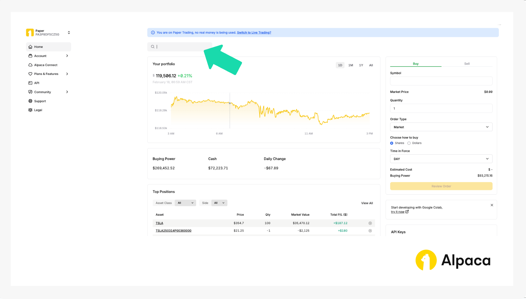
1. Log in to your account

Sign in to your account and navigate to the “Home” page.

2. Find your desired trade

On your dashboard in the top left, you can select between using your paper trading or live accounts. It’s important that you select the appropriate trading account before implementing an options strategy. If you want to practice without the risk of real capital, you can use your paper trading accounts. If you are looking to implement strategies, you can use your live account.

Once you’ve selected the desired account within your dashboard, you can monitor your portfolio, access market data, execute trades, and review your trading history. In order to create your first options trade, use the search bar to find and select the applicable option ticker symbol.

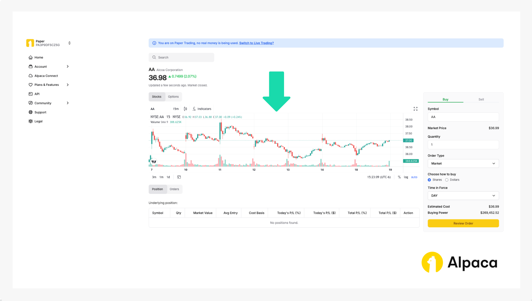
3. Check underlying security’s bar chart

If you search your desired underlying asset, a page shows the asset’s bar chart. You can use this bar chart for a simple analysis.

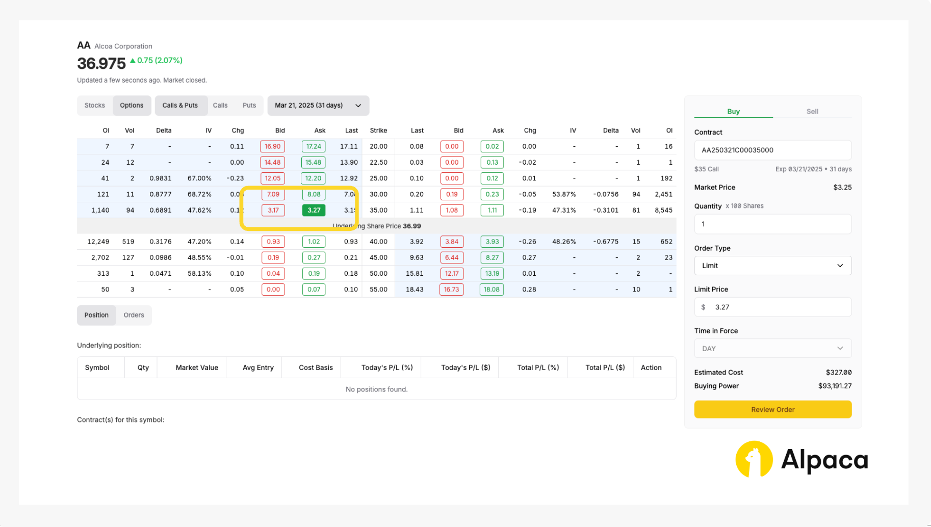
4. Opening an options position

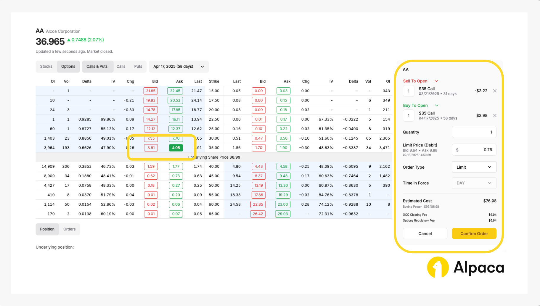
Assume we have already analyzed the market and determined the strike price for both a short call and a long call option to be $35.00. Once determined, select and review your order type (market or limit) and decide on the number of contracts you’d like to trade. You can select up to four legs. 

On the asset’s page, toggle from “Stocks” to “Options” and determine your desired contract type between calls and puts. You can also adjust the expiration date from the dropdown, ranging anywhere from 0DTE options to contracts hundreds of days in the future.

A long call calendar spread, for example, requires shorting a short-term call option and longing a long-term call option at the same strike price. Therefore, you can establish your position in the dashboard by selecting one short-term call option with “Sell To Open” and one long-term call option with “Buy To Open.” Click “Confirm Order” to purchase the options contracts.

Please note: The order in which you select the options does not matter. Additionally, on Alpaca’s dashboard and Trading API, credits are displayed as negative values, while debits appear as positive values. For example, in the image below, a debit spread (where your initial entry requires payment) is shown with a positive limit price ($0.76 in this case) under 'Limit Price (Debit),' reflecting a total debit of $76.08.

Once selected, review your order type (such as market, limit, stop, stop limit, or trailing stop) and the number of contracts you’d like to trade. Click the “Confirm Order” button on the bottom right.

Your paper trading account will then mimic the execution of the order as though it were a real transaction.

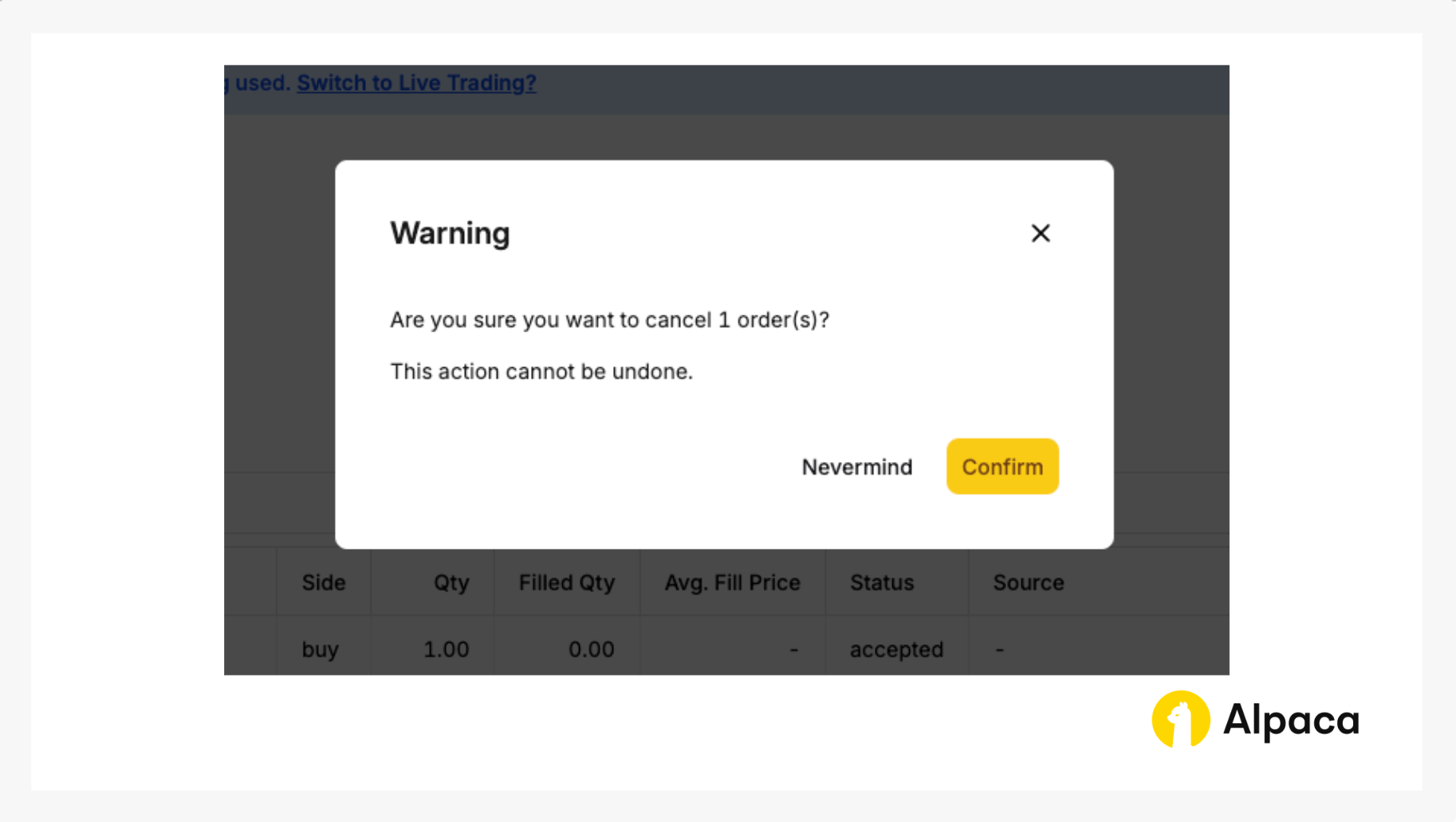
Optional: Cancel your order

Keep in mind that with multi-leg options order, you cannot cancel or replace a child leg individually. You can only cancel or replace your multi-leg options order as a whole.

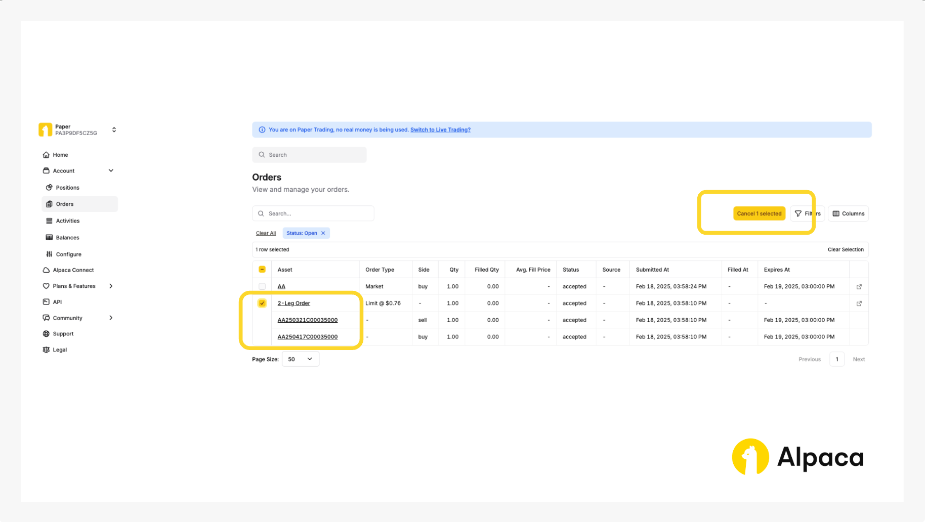
You’ll then be prompted to confirm.

5. Closing your position

Closing an options position involves selling the options contract that you previously bought (in a long position) or buying back the options contract that you previously sold (in a short position). Either action terminates, or “closes”, your associated position.

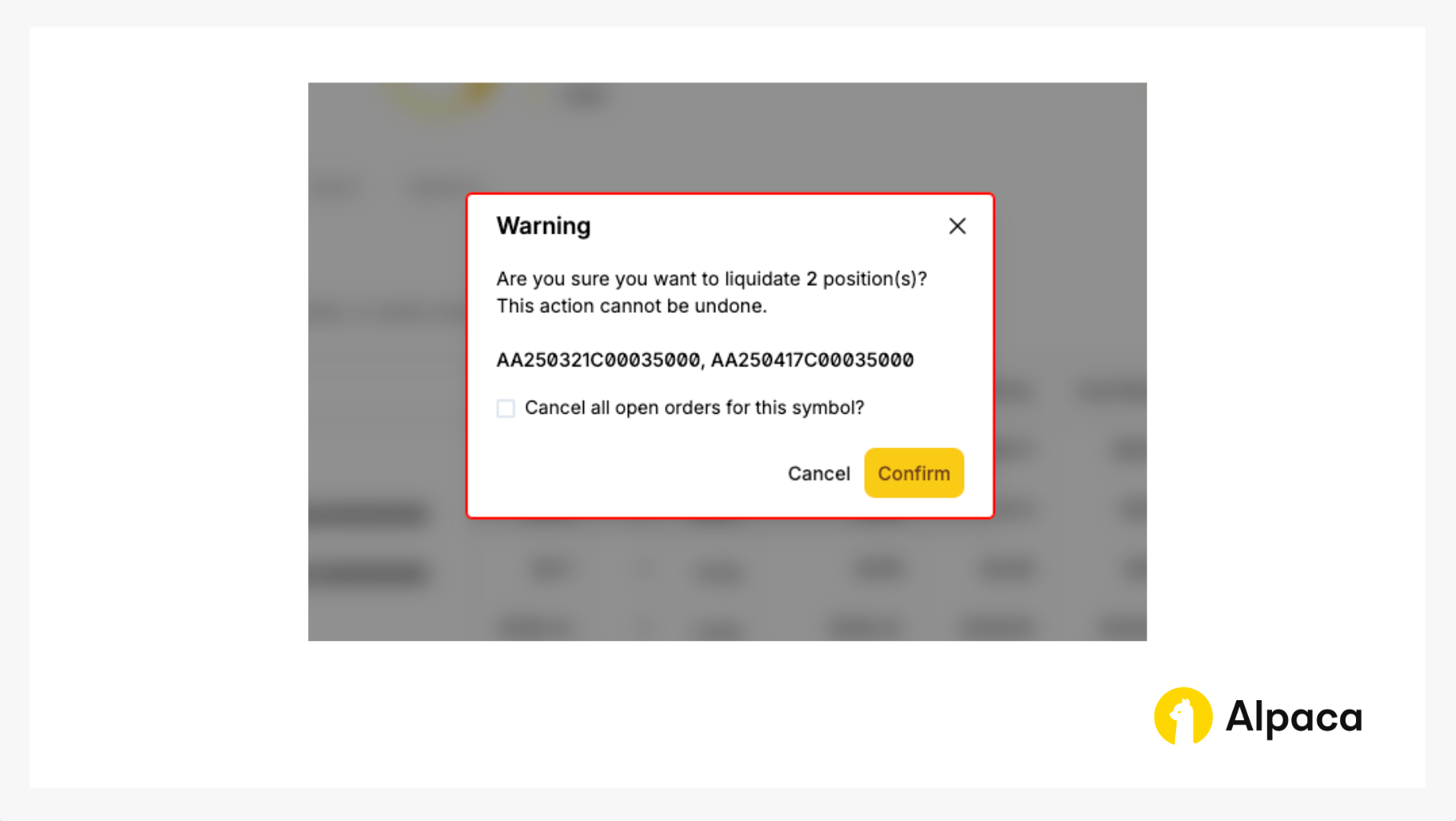
If you’d like to close your position, find the desired options contract on your “Home” page or under “Positions”. Click on the appropriate contract symbol and select “Close Position”.

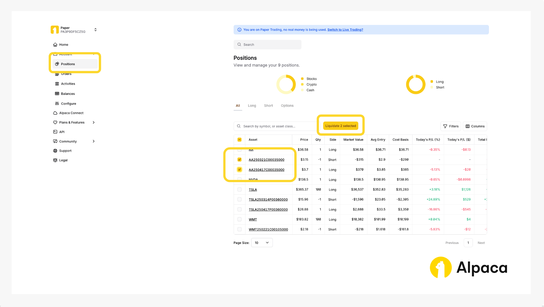
You will, then, click the “Confirm” button to liquidate the position.

How American-Style and European-Style Options Impact Calendar Spreads

The choice between American-style and European-style options affects the execution, pricing, and risk of calendar spreads. Traders and algorithmic developers may want to consider how these differences impact strategy performance.

American-Style Options

American-style options introduce early exercise risk, requiring adjustments if the short leg is assigned. This risk increases with dividends, interest rate changes, or significant price movements.

• Early Exercise: The short option would be assigned anytime before expiration.
• Dividend & Rate Sensitivity: Higher risk of early exercise near dividend dates.
• Adjustment Complexity: Unexpected assignments may disrupt strategy execution.

European-Style Options

European-style options simplify risk management since they can only be exercised at expiration, making them ideal for structured strategies.

• No Early Assignment: The short leg cannot be exercised before expiration.
• Predictable Decay & Volatility: More stable modeling of theta decay and vega.
• Easier Backtesting: Fixed expirations enable more precise historical simulations.

Understanding these differences helps traders align their strategies with their execution frameworks.

Adjustments in Algorithmic Trading

For algorithmic execution, American-style options require additional risk controls, while European-style options allow for more precise modeling.

• American-Style Algorithms:
  • Factor in early exercise risk, especially for short positions.
  • Account for dividend dates and assignment probabilities.
  • Use dynamic hedging or rolling adjustments.
  • Theoretical losses may not be accounted for, potentially leading to further losses.
• European-Style Algorithms:
  • Focus on time decay and volatility shifts without assignment risk.
  • Allow for more structured and systematic modeling.
  • Simplify integration into backtesting frameworks.

Choosing the right option type affects execution efficiency and risk management.

Conclusion

Calendar spreads offer a balanced way to capitalize on time decay and implied volatility—suited for both discretionary and algorithmic trading. When structured correctly, they may possibly generate recurring profit opportunities with defined risk. However, success hinges on accurately modeling volatility, managing early-assignment risk (particularly for American-style options), and making disciplined adjustments for market swings.

Backtesting across varied conditions is vital—whether you’re coding automated systems or trading manually. Combining robust data analytics, adaptive position sizing, and strategic rolling of the short leg helps you refine entries and exits. To get started with minimal risk, leverage Alpaca’s paper trading platform and comprehensive documentation. This hands-on approach will help you optimize calendar spreads before transitioning to live markets.

We hope you've found this tutorial on how to trade calendar spreads insightful and useful for getting started on your own strategy. As you put these concepts into practice, feel free to share your feedback and experiences on our forum, Slack community, or subreddit! And don’t forget to check out the rest of our options-related tutorials.

FAQs

Is a calendar spread bullish or bearish?

A calendar spread is typically a neutral strategy, aiming to profit from time decay and stable underlying asset prices. However, it can be tailored to a slightly bullish or bearish outlook depending on the choice between call or put options.

Are there other names for calendar spreads?

Yes, calendar spreads are also known as time spreads or horizontal spreads.

When should you exit a calendar spread?

You may want to consider exiting a calendar spread when:

• The underlying asset's price moves significantly away from the strike price.
• Implied volatility or option Greeks change unfavorably.
• The short-term option is nearing expiration, and maintaining the position no longer aligns with your market outlook.

Is a calendar spread a debit or credit spread?

It depends on whether you use a long calendar spread or a short calendar spread. A long calendar spread is typically a debit spread because the cost of the long-term option purchased usually exceeds the premium received from selling the short-term option, resulting in a net debit when establishing the position. Conversely, a short calendar spread is the opposite—it is primarily a credit spread.

Options trading is not suitable for all investors due to its inherent high risk, which can potentially result in significant losses. Please read Characteristics and Risks of Standardized Options before investing in options.

Past hypothetical backtest results do not guarantee future returns, and actual results may vary from the analysis.

The Paper Trading API is offered by AlpacaDB, Inc. and does not require real money or permit a user to transact in real securities in the market. Providing use of the Paper Trading API is not an offer or solicitation to buy or sell securities, securities derivative or futures products of any kind, or any type of trading or investment advice, recommendation or strategy, given or in any manner endorsed by AlpacaDB, Inc. or any AlpacaDB, Inc. affiliate and the information made available through the Paper Trading API is not an offer or solicitation of any kind in any jurisdiction where AlpacaDB, Inc. or any AlpacaDB, Inc. affiliate (collectively, “Alpaca”) is not authorized to do business.

Please note that this article is for general informational purposes only and is believed to be accurate as of the posting date but may be subject to change. The examples above are for illustrative purposes only.

All investments involve risk, and the past performance of a security, or financial product does not guarantee future results or returns. There is no guarantee that any investment strategy will achieve its objectives. Please note that diversification does not ensure a profit, or protect against loss. There is always the potential of losing money when you invest in securities, or other financial products. Investors should consider their investment objectives and risks carefully before investing.

Securities brokerage services are provided by Alpaca Securities LLC ("Alpaca Securities"), member FINRA/SIPC, a wholly-owned subsidiary of AlpacaDB, Inc. Technology and services are offered by AlpacaDB, Inc.

This is not an offer, solicitation of an offer, or advice to buy or sell securities or open a brokerage account in any jurisdiction where Alpaca Securities are not registered or licensed, as applicable.